|
|
|
|
•
|
|
•
|
|
•
|
|
•
|
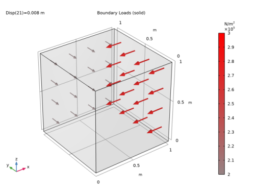
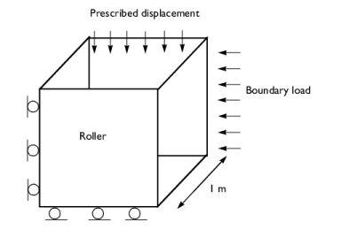
On the other two vertical walls (x = 1 m and y = 1 m), apply boundary loads of 300 kPa and 200 kPa, as shown on Figure 2.
|
|
1
|
|
2
|
|
3
|
Click Add.
|
|
4
|
Click
|
|
5
|
|
6
|
Click
|
|
1
|
|
2
|
|
1
|
|
2
|
|
3
|
|
1
|
|
2
|
|
3
|
|
1
|
|
2
|
|
3
|
From the list, choose Diagonal.
|
|
4
|
|
1
|
|
1
|
|
3
|
|
4
|
|
1
|
|
3
|
|
4
|
|
1
|
|
3
|
|
4
|
|
5
|
|
1
|
In the Model Builder window, under Component 1 (comp1) right-click Materials and choose Blank Material.
|
|
2
|
|
1
|
|
1
|
|
2
|
|
3
|
|
4
|
|
1
|
|
2
|
|
3
|
|
4
|
Click
|
|
6
|
|
1
|
|
1
|
|
2
|
|
3
|
|
4
|
|
5
|
In the associated text field, type Vertical displacement (mm).
|
|
6
|
|
7
|
In the associated text field, type Stress (kPa).
|
|
1
|
|
3
|
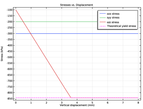
In the Settings window for Point Graph, click Replace Expression in the upper-right corner of the y-Axis Data section. From the menu, choose Component 1 (comp1)>Solid Mechanics>Stress>Stress tensor (spatial frame) - N/m²>solid.sx - Stress tensor, x component.
|
|
4
|
|
5
|
|
6
|
|
7
|
Click to expand the Coloring and Style section. Click to expand the Legends section. Select the Show legends check box.
|
|
8
|
|
10
|
|
1
|
|
2
|
In the Settings window for Point Graph, click Replace Expression in the upper-right corner of the y-Axis Data section. From the menu, choose Component 1 (comp1)>Solid Mechanics>Stress>Stress tensor (spatial frame) - N/m²>solid.sy - Stress tensor, y component.
|
|
3
|
|
4
|
Locate the Legends section. In the table, enter the following settings:
|
|
1
|
In the Model Builder window, under Results>Stresses vs. Displacement right-click Point Graph 1 and choose Duplicate.
|
|
2
|
In the Settings window for Point Graph, click Replace Expression in the upper-right corner of the y-Axis Data section. From the menu, choose Component 1 (comp1)>Solid Mechanics>Stress>Stress tensor (spatial frame) - N/m²>solid.sz - Stress tensor, z component.
|
|
3
|
|
4
|
Locate the Legends section. In the table, enter the following settings:
|
|
1
|
|
2
|
|
3
|
In the Expression text field, type (2*solid.cohesion*cos(solid.internalphi)-Y_stress*(1+sin(solid.internalphi)))/(sin(solid.internalphi)-1).
|
|
4
|
Locate the Coloring and Style section. Find the Line style subsection. From the Line list, choose Dashed.
|
|
5
|
|
6
|
Locate the Legends section. In the table, enter the following settings:
|
|
7
|