|
|
|


|
1
|
|
2
|
|
3
|
Click Add.
|
|
4
|
Click
|
|
5
|
|
6
|
Click
|
|
1
|
|
2
|
|
3
|
|
1
|
|
2
|
|
1
|
|
2
|
|
3
|
|
4
|
|
5
|
|
1
|
|
2
|
On the object pol1, select Point 3 only.
|
|
3
|
|
4
|
|
5
|
|
1
|
|
2
|
|
3
|
|
4
|
Locate the Revolution Axis section. Find the Direction of revolution axis subsection. In the xw text field, type 1.
|
|
5
|
|
6
|
|
1
|
In the Model Builder window, under Component 1 (comp1) right-click Solid Mechanics (solid) and choose Fixed Constraint.
|
|
1
|
|
1
|
|
2
|
|
3
|
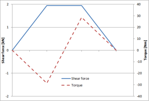
Specify the F vector as
|
|
4
|
|
1
|
|
2
|
|
3
|
Specify the M vector as
|
|
4
|
|
1
|
In the Model Builder window, under Global Definitions>Load and Constraint Groups click Load Group 1.
|
|
2
|
|
3
|
|
1
|
In the Model Builder window, under Global Definitions>Load and Constraint Groups click Load Group 2.
|
|
2
|
|
3
|
|
1
|
In the Model Builder window, under Component 1 (comp1) right-click Materials and choose Blank Material.
|
|
2
|
|
1
|
|
2
|
|
3
|
|
4
|
|
5
|
|
1
|
|
2
|
|
3
|
|
1
|
|
2
|
|
3
|
|
5
|
|
6
|
|
8
|
|
10
|
|
1
|
|
2
|
|
3
|
|
4
|
Click Add two times.
|
|
6
|
|
7
|
|
8
|
|
1
|
|
2
|
|
3
|
|
1
|
|
2
|
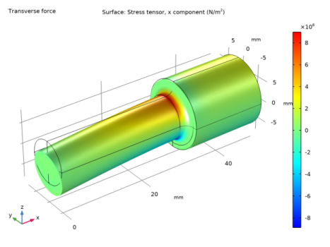
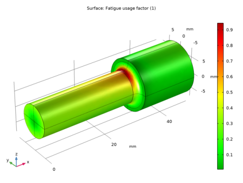
In the Settings window for Surface, click Replace Expression in the upper-right corner of the Expression section. From the menu, choose Component 1 (comp1)>Solid Mechanics>Stress>Stress tensor (spatial frame) - N/m²>solid.sx - Stress tensor, x component.
|
|
3
|
|
1
|
|
2
|
|
3
|
|
4
|
|
5
|
|
1
|
|
2
|
|
3
|
Click Add three times.
|
|
5
|
|
6
|
|
7
|
|
1
|
|
2
|
|
1
|
|
2
|
|
3
|
|
4
|
Find the Physics interfaces in study subsection. In the table, clear the Solve check boxes for Study 1 (Basic load cases) and Study 2 (Combined load cases).
|
|
5
|
|
6
|
|
1
|
|
2
|
|
3
|
|
4
|
|
5
|
|
1
|
|
2
|
|
3
|
|
4
|
|
5
|
|
6
|
|
1
|
|
2
|
|
3
|
|
4
|
|
5
|
|
1
|
In the Model Builder window, under Component 1 (comp1) right-click Materials and choose Blank Material.
|
|
2
|
|
3
|
|
4
|
|
5
|
|
1
|
|
2
|
|
3
|
Find the Physics interfaces in study subsection. In the table, clear the Solve check box for Solid Mechanics (solid).
|
|
4
|
Find the Studies subsection. In the Select Study tree, select Preset Studies for Selected Physics Interfaces>Fatigue.
|
|
5
|
|
6
|
|
1
|
|
2
|
Find the Values of variables not solved for subsection. From the Settings list, choose User controlled.
|
|
3
|
|
4
|
|
5
|
|
6
|
|
7
|
|
1
|
|
2
|
|
3
|
|
1
|
|
2
|
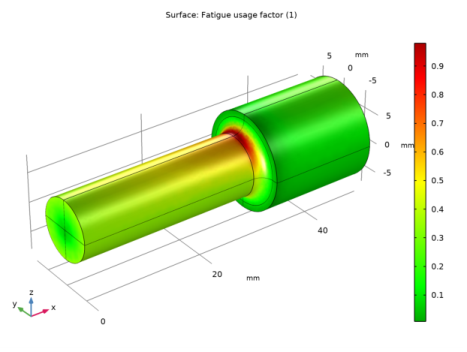
In the Settings window for 3D Plot Group, type Fatigue Usage Factor (Matake) in the Label text field.
|
|
1
|
|
2
|
|
3
|
|
1
|
|
2
|
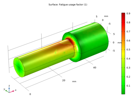
In the Settings window for 3D Plot Group, type Fatigue Usage Factor (Dang Van) in the Label text field.
|
|
1
|
|
2
|
|
3
|
|
1
|
|
2
|
|
3
|
|
4
|
|
5
|
|
1
|
|
3
|
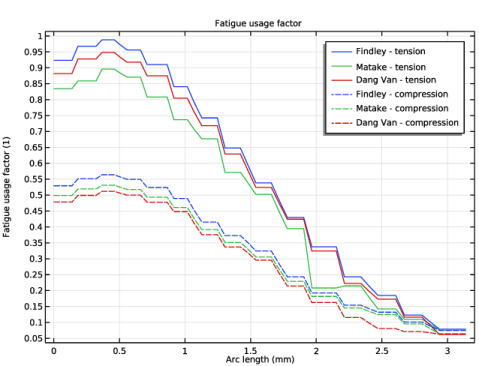
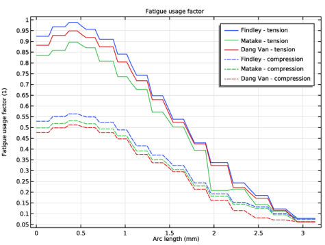
In the Settings window for Line Graph, click Replace Expression in the upper-right corner of the y-Axis Data section. From the menu, choose Component 1 (comp1)>Fatigue>ftg.stre1.fus - Fatigue usage factor.
|
|
4
|
|
5
|
|
1
|
|
2
|
|
3
|
|
4
|
Locate the Legends section. In the table, enter the following settings:
|
|
1
|
|
2
|
|
3
|
|
4
|
Locate the Legends section. In the table, enter the following settings:
|
|
1
|
|
3
|
In the Settings window for Line Graph, click Replace Expression in the upper-right corner of the y-Axis Data section. From the menu, choose ftg.stre1.fus - Fatigue usage factor.
|
|
4
|
Click to expand the Coloring and Style section. Find the Line style subsection. From the Line list, choose Dashed.
|
|
5
|
|
6
|
|
7
|
|
1
|
|
2
|
|
3
|
|
4
|
|
5
|
Locate the Legends section. In the table, enter the following settings:
|
|
1
|
|
2
|
|
3
|
|
4
|
Locate the Legends section. In the table, enter the following settings:
|
|
5
|