|
|
|
|
1
|
|
2
|
From the Application Libraries root, browse to the folder Structural_Mechanics_Module/Tutorials and double-click the file bracket_spring.mph.
|
|
1
|
|
2
|
|
1
|
In the Model Builder window, expand the Component 1 (comp1)>Definitions node, then click Analytic 1 (load).
|
|
2
|
|
3
|
|
1
|
|
2
|
|
3
|
|
4
|
|
6
|
|
7
|
|
8
|
|
9
|
|
1
|
|
2
|
|
3
|
|
4
|
Click
|
|
6
|
|
1
|
|
2
|
|
3
|
|
4
|
Find the Functions subsection. In the table, enter the following settings:
|
|
5
|
Click Browse.
|
|
6
|
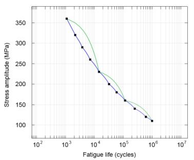
Browse to the model’s Application Libraries folder and double-click the file bracket_fatigue_sn_curve.txt.
|
|
7
|
Click Import.
|
|
1
|
|
2
|
|
3
|
Find the Physics interfaces in study subsection. In the table, clear the Solve check box for Study 1.
|
|
4
|
|
5
|
|
6
|
|
1
|
|
2
|
|
3
|
|
4
|
|
5
|
|
6
|
|
7
|
|
8
|
|
9
|
|
1
|
|
2
|
|
3
|
Find the Physics interfaces in study subsection. In the table, clear the Solve check box for Solid Mechanics (solid).
|
|
4
|
Find the Studies subsection. In the Select Study tree, select Preset Studies for Selected Physics Interfaces>Fatigue.
|
|
5
|
|
6
|
|
1
|
|
2
|
Find the Values of variables not solved for subsection. From the Settings list, choose User controlled.
|
|
3
|
|
4
|
|
1
|
|
2
|
|
3
|
Click
|
|
5
|
|
1
|
|
2
|
|
3
|
|
4
|
|
5
|
|
6
|
Click OK.
|
|
1
|
|
3
|
|
4
|
|
1
|
|
2
|
|
3
|
|
4
|
|
1
|
|
2
|
|
3
|
|
4
|
|
1
|
|
2
|