PDF

Accelerated Life Testing
Introduction
Fatigue testing of nonlinear materials with a creep mechanism is a time consuming process. In accelerated life testing, the experiment time is greatly reduced by subjecting the material to testing conditions in excess of the operating ones. In this model an aggressive thermal load cycle is simulated and, its effect on the fatigue life of a solder joint is examined.
This example demonstrates how to evaluate fatigue driven by a specific strain or energy quantity and therefore a simple schematic representation of an electronic component is used. Moreover, only one cycle is simulated as opposed to several that are required to obtain a steady state cycle when working with nonlinear materials. This simplification is motivated by the fact that the purpose of this model is to show how to evaluate fatigue based on a user defined variable. The required strain and energy variables are defined explicitly via ordinary differential equations and calculated during the simulation of the thermal load cycle.
Model Definition
Microelectronic components consist of several materials. When subjected to temperature changes, differences in coefficients of thermal expansion introduce a stress concentration caused by the discontinuous deformation. With consecutive heating and cooling, the stress state changes back and forth until the component finally fails in fatigue.
This example uses a schematic geometry which captures the structural function of the main components rather than an accurate geometry of the microelectronic component. A symmetric model is used and half of its geometry is shown in Figure 1. The total size of the resistor and of the printed circuit board (PCB) is 4 × 0.5 mm2. The size of the solder is 0.5 × 0.25 mm2. It is assumed that the structure is in plane strain conditions.
The resistor is made of alumina, the printed circuit board is a fiberglass based laminate and the solder joint is an SnAgCu alloy that responds both linearly and nonlinearly to an applied load. The elastic and the thermal properties of the materials are given in Table 1.
Figure 1: Geometry of the electronic component. The dashed line indicates symmetry.
The solder material nonlinearity is creep, which is a material behavior where deformation changes over the time although the stress remain constant. Generally materials creep with different rates in three distinct phases: primary creep, secondary creep and tertiary creep; see Figure 2.
Figure 2: Creep strain development at constant stress. Primary creep denoted with 1, secondary with 2 and tertiary with 3.
The secondary creep is also called the steady state creep since the strain rate at constant stress is constant. In the representation of the solder material the primary and tertiary creeps are disregarded while the steady state creep is represented with a double Norton law according to
where is the creep rate, σe is the equivalent stress and AI, nI, σn, AII, and nII are the material constants given by Table 2. The first term represents a creep mechanism observed at low stresses while the second term describes the dominating creep behavior at high stresses, see Figure 3.
AI
8.03·10-12 1/s
nI
σn
AII
1.96·10-23 1/s
nII
Figure 3: Creep model for the solder SnAgCu solder material.
Two fatigue models are evaluated. In the first, the lifetime is based on a Coffin-Manson type model. The development of the shear strain controls the fatigue according to
where ΔγII is the range of the creep shear strain of the second creep mechanism experienced in a load cycle and N is the number of cycles to fatigue.
The second fatigue evaluation depends on the energy dissipation and follows a Morrow type criterion according expressed as
where ΔWII is the dissipated creep energy of the second creep mechanism during a load cycle.
Results and Discussion
First the user defined creep strains and energies are verified. The creep strain calculated in the structural analysis is a summation of creep contributions from different mechanisms and thus
where is the creep strain of the first mechanism and is the creep strain contribution from the second mechanism. The individual contributions of each creep mechanism are calculated in two separate ODE interfaces. A composition of creep results is shown in Figure 4.
Figure 4: Creep strain history. The equivalent creep strain is shown.
From the figure it is clear that the creep strain calculated using the Nonlinear Structural Materials Module equals the sum of the creep strains calculated with the user defined method.
The creep energy dissipation can also be calculated using the additive decomposition since
where δ denotes an increment and Wc denotes the energy dissipation density. The results of the energy comparison in Figure 5 shows a perfect agreement between values calculated by the built-in materials and the user defined material.
Figure 5: The energy dissipation history.
The fatigue lives predicted by the Coffin-Manson type model and the Morrow type model are shown in Figure 6 and Figure 7 respectively. The predicted life differs by approximately a factor of two, which is not uncommon when using fatigue models of different types, with some uncertainty in the model parameters. Both models indicate that the upper left corner is the critical point in the assembly.
Figure 6: Fatigue life based on the shear strain.
Figure 7: Fatigue life based on the dissipated energy.
Notes About the COMSOL Implementation
Fatigue can be evaluated using many different models. Several models share the same mathematical form. This is the case for the Coffin-Manson based and Morrow based models where the only difference is the controlling strain or energy measure. In rocks and rubbers it is commonly the elastic strain energy or the total strain energy that controls fatigue while in materials subjected to cyclic creep, the dissipated energy controls the fatigue. The Coffin-Manson model that initially related plastic strain to fatigue life has been modified by several researchers that propose a variety of different strain measures as the fatigue controlling mechanism.
In COMSOL Multiphysics, the Morrow and the Coffin-Manson relations
can be modified so that the fatigue evaluation is based on a user defined energy density, W, or strain, ε. If the variable controlling fatigue is already defined in a physics interface, it can be directly specified in the fatigue model node. The variable must be specified together with the corresponding physics interface tag (for example, solid.Ws when using the elastic strain energy density). When the variable is not defined in a physics interface, it can be calculated using an ODE Interface. This procedure is demonstrated in this model, where the fatigue is dependent on a specific creep strain and a specific dissipated energy density.
The basic form for an ODE is
(1)
where u is the field variable, t is the time, ea denotes the mass coefficient matrix, da denotes the damping coefficient matrix and f is the source term. The development of creep following the Norton’s law is defined with
(2)
where ij denotes a specific component, σe is the effective von Mises stress, sij is the deviatoric stress, and A, σref and n are material constants. Since the problem is a 2D plane stress analysis, only strains in x, y, z, and xy directions can develop. This gives 4 dependent variables: ecx, ecy, ecz, and ecxy. By comparing the first relation of Equation 2 with Equation 1 it can be identified that there is no contribution from the mass matrix, the damping matrix is an identity matrix and the source term equals the right-hand side of the first relation in Equation 2. This relation contains both the deviatoric stress tensor and the equivalent stress. Since both are already defined in the Solid Mechanics interface, it seems that they can be used in the definition of the source term. COMSOL Multiphysics requires, however, that the derivatives of all user-defined variables can be evaluated at all calculation steps of the analysis. At zero stress the numerical derivative of the equivalent stress
tries to evaluate a negative power of zero. A remedy to this challenge is to provide your own definition of the equivalent stress with a small addition of stress.
The nonzero stress ensures a finite derivative at stress free conditions. In the example a stress addition of 1Pa was chosen. This gives a negligible contribution to the equivalent stress since the resulting stresses have the order of magnitude of MPa.
In addition to the dependent variables used for the creep strain components, one additional dependent variable, ece, for the equivalent creep strain as defined by the second relation in Equation 2 is needed. The source term for this relation can be defined using the built-in derivative operator in COMSOL Multiphysics. For example a partial derivative of u with respect to x is simply defined as d(u,x). By putting all together, the time derivatives of the five dependent variables ecx, ecy, ecz, ecxy, and ece become:
alpha*solid.sdevx
alpha*solid.sdevy
alpha*solid.sdevz
alpha*solid.sdevxy
(2/3*(d(ecx,TIME)^2+d(ecy,TIME)^2+d(ecz,TIME)^2+2*(d(ecxy,TIME)^2))+1e-20)^0.5
where alpha=3/2*A/s_mises*(s_mises/s_ref)^n and s_mises=sqrt(solid.sx^2+solid.sy^2+solid.sz^2-solid.sx*solid.sy-solid.sy*solid.sz-solid.sz*solid.sx+3*solid.sxy^2+(1e-6[MPa])^2).
The time derivative of the dissipated creep energy density is
By using the derivative operator, the source term for the dependent variable, Wc, is simply d(ece,TIME)*s_mises.
The calculation of the strain variables and the energy density must be made in separate ODE Interfaces since the units of both variables differ.
Application Library path: Fatigue_Module/Strain_Life/accelerated_life_testing
Modeling Instructions
From the File menu, choose New.
New
In the New window, click  Blank Model.
Add Component
In the Home toolbar, click  Add Component and choose 2D.
Geometry 1
1
In the Settings window for Geometry, locate the Units section.
2
From the Length unit list, choose mm.
Rectangle 1 (r1)
1
In the Geometry toolbar, click  Rectangle.
2
In the Settings window for Rectangle, locate the Size and Shape section.
3
In the Width text field, type 2.
4
In the Height text field, type 0.5.
Rectangle 2 (r2)
1
In the Geometry toolbar, click  Rectangle.
2
In the Settings window for Rectangle, locate the Size and Shape section.
3
In the Width text field, type 0.5.
4
In the Height text field, type 0.25.
5
Locate the Position section. In the y text field, type 0.5.
Rectangle 3 (r3)
1
In the Geometry toolbar, click  Rectangle.
2
In the Settings window for Rectangle, locate the Size and Shape section.
3
In the Width text field, type 2.
4
In the Height text field, type 0.5.
5
Locate the Position section. In the y text field, type 0.75.
Point 1 (pt1)
1
In the Geometry toolbar, click  Point.
2
In the Settings window for Point, locate the Point section.
3
In the x text field, type 0.25.
4
In the y text field, type 0.625.
5
Click  Build Selected.
6
Click the  Zoom Extents button in the Graphics toolbar.
Add Physics
1
In the Home toolbar, click  Add Physics to open the Add Physics window.
2
Go to the Add Physics window.
3
In the tree, select Structural Mechanics>Solid Mechanics (solid).
4
Click Add to Component 1 in the window toolbar.
5
In the Home toolbar, click  Add Physics to close the Add Physics window.
Global Definitions
Parameters 1
1
In the Model Builder window, under Global Definitions click Parameters 1.
2
In the Settings window for Parameters, locate the Parameters section.
3
Interpolation 1 (int1)
1
In the Home toolbar, click  Functions and choose Global>Interpolation.
2
In the Settings window for Interpolation, locate the Definition section.
3
In the Function name text field, type thermLC.
4
5
Locate the Units section. In the Arguments text field, type min.
6
In the Function text field, type degC.
Solid Mechanics (solid)
Linear Elastic Material 1
1
Click the  Show More Options button in the Model Builder toolbar.
2
In the Show More Options dialog box, in the tree, select the check box for the node Physics>Advanced Physics Options.
3
4
In the Model Builder window, under Component 1 (comp1)>Solid Mechanics (solid) click Linear Elastic Material 1.
5
In the Settings window for Linear Elastic Material, click to expand the Energy Dissipation section.
6
Select the Calculate dissipated energy check box.
Thermal Expansion 1
1
In the Physics toolbar, click  Attributes and choose Thermal Expansion.
2
In the Settings window for Thermal Expansion, locate the Model Input section.
3
From the T list, choose User defined. In the associated text field, type thermLC(t).
Linear Elastic Material 1
In the Model Builder window, click Linear Elastic Material 1.
Creep 1
1
In the Physics toolbar, click  Attributes and choose Creep.
2
3
In the Settings window for Creep, locate the Creep Data section.
4
From the A list, choose User defined. In the associated text field, type A_I.
5
From the σref list, choose User defined. In the associated text field, type s_ref.
6
From the n list, choose User defined. In the associated text field, type n_I.
Linear Elastic Material 1
In the Model Builder window, click Linear Elastic Material 1.
Creep 2
1
In the Physics toolbar, click  Attributes and choose Creep.
2
3
In the Settings window for Creep, locate the Creep Data section.
4
From the A list, choose User defined. In the associated text field, type A_II.
5
From the σref list, choose User defined. In the associated text field, type s_ref.
6
From the n list, choose User defined. In the associated text field, type n_II.
Symmetry 1
1
In the Physics toolbar, click  Boundaries and choose Symmetry.
2
Fixed Constraint 1
1
In the Physics toolbar, click  Points and choose Fixed Constraint.
2
Materials
PCB
1
In the Model Builder window, under Component 1 (comp1) right-click Materials and choose Blank Material.
2
In the Settings window for Material, type PCB in the Label text field.
3
4
Locate the Material Contents section. In the table, enter the following settings:
Solder
1
Right-click Materials and choose Blank Material.
2
In the Settings window for Material, type Solder in the Label text field.
3
4
Locate the Material Contents section. In the table, enter the following settings:
Alumina
1
Right-click Materials and choose Blank Material.
2
In the Settings window for Material, type Alumina in the Label text field.
3
4
Locate the Material Contents section. In the table, enter the following settings:
Definitions
Variables 1
1
In the Model Builder window, under Component 1 (comp1) right-click Definitions and choose Variables.
Define help variables for the user defined strains.
2
In the Settings window for Variables, locate the Variables section.
3
Add Physics
1
In the Physics toolbar, click  Add Physics to open the Add Physics window.
2
Go to the Add Physics window.
3
In the tree, select Mathematics>ODE and DAE Interfaces>Domain ODEs and DAEs (dode).
4
Click Add to Component 1 in the window toolbar.
5
In the tree, select Recently Used>Domain ODEs and DAEs (dode).
6
Click Add to Component 1 in the window toolbar.
7
In the tree, select Recently Used>Domain ODEs and DAEs (dode).
8
Click Add to Component 1 in the window toolbar.
9
In the Physics toolbar, click  Add Physics to close the Add Physics window.
Domain ODEs and DAEs (dode)
1
In the Model Builder window, under Component 1 (comp1) click Domain ODEs and DAEs (dode).
2
3
In the Settings window for Domain ODEs and DAEs, locate the Units section.
4
In the Source term quantity table, enter the following settings:
5
Click to expand the Dependent Variables section. In the Field name text field, type ec_I.
6
In the Number of dependent variables text field, type 5.
7
In the Dependent variables table, enter the following settings:
Set the same Gauss point integration order as in the built-in Norton material.
8
Click to expand the Discretization section. From the Shape function type list, choose Gauss point data.
9
From the Element order list, choose 4.
Distributed ODE 1
1
In the Model Builder window, under Component 1 (comp1)>Domain ODEs and DAEs (dode) click Distributed ODE 1.
2
In the Settings window for Distributed ODE, locate the Source Term section.
3
In the f text-field array, type alpha_I*solid.sdevx on the first row.
4
In the f text-field array, type alpha_I*solid.sdevy on the second row.
5
In the f text-field array, type alpha_I*solid.sdevz on the third row.
6
In the f text-field array, type alpha_I*solid.sdevxy on the fourth row.
7
2/3*(d(ecx_I,TIME)^2+d(ecy_I,TIME)^2+d(ecz_I,TIME)^2+
2*(d(ecxy_I,TIME)^2))+(1e-20))^0.5
on the 5th row.
Domain ODEs and DAEs 2 (dode2)
1
In the Model Builder window, under Component 1 (comp1) click Domain ODEs and DAEs 2 (dode2).
2
3
In the Settings window for Domain ODEs and DAEs, locate the Units section.
4
In the Source term quantity table, enter the following settings:
5
Locate the Dependent Variables section. In the Field name text field, type ec_II.
6
In the Number of dependent variables text field, type 5.
7
In the Dependent variables table, enter the following settings:
8
Locate the Discretization section. From the Shape function type list, choose Gauss point data.
9
From the Element order list, choose 4.
Distributed ODE 1
1
In the Model Builder window, click Distributed ODE 1.
2
In the Settings window for Distributed ODE, locate the Source Term section.
3
In the f text-field array, type alpha_II*solid.sdevx on the first row.
4
In the f text-field array, type alpha_II*solid.sdevy on the second row.
5
In the f text-field array, type alpha_II*solid.sdevz on the third row.
6
In the f text-field array, type alpha_II*solid.sdevxy on the fourth row.
7
2/3*(d(ecx_II,TIME)^2+d(ecy_II,TIME)^2+d(ecz_II,TIME)^2+
2*(d(ecxy_II,TIME)^2))+(1e-20))^0.5
on the 5th row.
Domain ODEs and DAEs 3 (dode3)
1
In the Model Builder window, under Component 1 (comp1) click Domain ODEs and DAEs 3 (dode3).
2
3
In the Settings window for Domain ODEs and DAEs, locate the Units section.
4
Click  Select Dependent Variable Quantity.
5
In the Physical Quantity dialog box, type energydensity in the text field.
6
Click  Filter.
7
In the tree, select Electromagnetics>Energy density (J/m^3).
8
9
In the Settings window for Domain ODEs and DAEs, locate the Units section.
10
In the Source term quantity table, enter the following settings:
11
Locate the Dependent Variables section. In the Field name text field, type Wc.
12
In the Number of dependent variables text field, type 2.
13
In the Dependent variables table, enter the following settings:
14
Locate the Discretization section. From the Shape function type list, choose Gauss point data.
15
From the Element order list, choose 4.
Distributed ODE 1
1
In the Model Builder window, click Distributed ODE 1.
2
In the Settings window for Distributed ODE, locate the Source Term section.
3
In the f text-field array, type d(ece_I,TIME)*s_mises on the first row.
4
In the f text-field array, type d(ece_II,TIME)*s_mises on the second row.
Mesh 1
Free Triangular 1
In the Mesh toolbar, click  Free Triangular.
Size 1
1
Right-click Free Triangular 1 and choose Size.
2
In the Settings window for Size, locate the Geometric Entity Selection section.
3
From the Geometric entity level list, choose Domain.
4
5
Locate the Element Size section. From the Predefined list, choose Finer.
6
Click  Build All.
Add Study
1
In the Home toolbar, click  Add Study to open the Add Study window.
2
Go to the Add Study window.
3
Find the Studies subsection. In the Select Study tree, select General Studies>Time Dependent.
4
Click Add Study in the window toolbar.
5
In the Home toolbar, click  Add Study to close the Add Study window.
Study 1
Step 1: Time Dependent
1
In the Settings window for Time Dependent, locate the Study Settings section.
2
From the Time unit list, choose min.
3
In the Output times text field, type range(0,0.5,14.5) range(14.6,0.1,15.4) range(15.5,0.5,29.5) range(29.6,0.1,30.4) range(30.5,0.5,44.5) range(44.6,0.1,45.4) range(45.5,0.5,60).
Solution 1 (sol1)
1
In the Study toolbar, click  Show Default Solver.
2
In the Model Builder window, expand the Solution 1 (sol1) node, then click Time-Dependent Solver 1.
3
In the Settings window for Time-Dependent Solver, click to expand the Time Stepping section.
4
From the Steps taken by solver list, choose Intermediate.
5
In the Study toolbar, click  Compute.
Results
Stress (solid)
Click the  Zoom Extents button in the Graphics toolbar.
Creep strain I (dode)
1
In the Model Builder window, under Results click 2D Plot Group 3.
2
In the Settings window for 2D Plot Group, type Creep strain I (dode) in the Label text field.
Surface 1
1
In the Model Builder window, expand the Creep strain I (dode) node, then click Surface 1.
2
In the Settings window for Surface, locate the Expression section.
3
In the Expression text field, type ece_I.
Creep strain II (dode2)
1
In the Model Builder window, expand the Results>2D Plot Group 4 node, then click 2D Plot Group 4.
2
In the Settings window for 2D Plot Group, type Creep strain II (dode2) in the Label text field.
Surface 1
1
In the Model Builder window, click Surface 1.
2
In the Settings window for Surface, locate the Expression section.
3
In the Expression text field, type ece_II.
Dissipated energy (dode3)
1
In the Model Builder window, under Results click 2D Plot Group 5.
2
In the Settings window for 2D Plot Group, type Dissipated energy (dode3) in the Label text field.
Create a plot that shows how strain develops during one cycle.
Creep strain history
1
In the Home toolbar, click  Add Plot Group and choose 1D Plot Group.
2
In the Settings window for 1D Plot Group, type Creep strain history in the Label text field.
Point Graph 1
1
Right-click Creep strain history and choose Point Graph.
2
3
In the Settings window for Point Graph, locate the y-Axis Data section.
4
In the Expression text field, type solid.ecGp11.
5
Click to expand the Legends section. Select the Show legends check box.
6
From the Legends list, choose Manual.
7
Point Graph 2
1
Right-click Point Graph 1 and choose Duplicate.
2
In the Settings window for Point Graph, locate the y-Axis Data section.
3
In the Expression text field, type solid.ecGp22.
4
Locate the Legends section. In the table, enter the following settings:
Point Graph 3
1
Right-click Point Graph 2 and choose Duplicate.
2
In the Settings window for Point Graph, locate the y-Axis Data section.
3
In the Expression text field, type solid.ecGp33.
4
Locate the Legends section. In the table, enter the following settings:
Point Graph 4
1
Right-click Point Graph 3 and choose Duplicate.
2
In the Settings window for Point Graph, locate the y-Axis Data section.
3
In the Expression text field, type solid.ecGp12.
4
Locate the Legends section. In the table, enter the following settings:
Creep strain history
1
In the Model Builder window, click Creep strain history.
2
In the Settings window for 1D Plot Group, locate the Legend section.
3
From the Position list, choose Lower right.
4
Click to expand the Title section. From the Title type list, choose None.
5
Locate the Plot Settings section. Select the y-axis label check box.
6
Verify that strains and energies are correctly calculated in the analysis.
1D Plot Group 7
In the Home toolbar, click  Add Plot Group and choose 1D Plot Group.
Point Graph 1
1
Right-click 1D Plot Group 7 and choose Point Graph.
2
In the Settings window for Point Graph, locate the y-Axis Data section.
3
In the Expression text field, type solid.eceGp.
4
5
Locate the Legends section. Select the Show legends check box.
6
From the Legends list, choose Manual.
7
Point Graph 2
1
Right-click Point Graph 1 and choose Duplicate.
2
In the Settings window for Point Graph, locate the y-Axis Data section.
3
In the Expression text field, type ece_I.
4
Locate the Legends section. In the table, enter the following settings:
Point Graph 3
1
Right-click Point Graph 2 and choose Duplicate.
2
In the Settings window for Point Graph, locate the y-Axis Data section.
3
In the Expression text field, type ece_II.
4
Locate the Legends section. In the table, enter the following settings:
Point Graph 4
1
Right-click Point Graph 3 and choose Duplicate.
2
In the Settings window for Point Graph, locate the y-Axis Data section.
3
In the Expression text field, type ece_I+ece_II.
4
Locate the Legends section. In the table, enter the following settings:
5
Click to expand the Coloring and Style section. Find the Line style subsection. From the Line list, choose Dotted.
6
In the Width text field, type 4.
Effective creep history
1
In the Model Builder window, under Results click 1D Plot Group 7.
2
In the Settings window for 1D Plot Group, type Effective creep history in the Label text field.
3
Locate the Legend section. From the Position list, choose Upper left.
4
Locate the Title section. From the Title type list, choose None.
5
Locate the Plot Settings section. Select the y-axis label check box.
6
In the associated text field, type Effective creep strain (1).
Creep dissipation history
1
Right-click Effective creep history and choose Duplicate.
2
In the Settings window for 1D Plot Group, type Creep dissipation history in the Label text field.
Point Graph 1
1
In the Model Builder window, expand the Creep dissipation history node, then click Point Graph 1.
2
In the Settings window for Point Graph, locate the y-Axis Data section.
3
In the Expression text field, type solid.Wc.
4
Locate the Legends section. In the table, enter the following settings:
Point Graph 2
1
In the Model Builder window, click Point Graph 2.
2
In the Settings window for Point Graph, locate the y-Axis Data section.
3
In the Expression text field, type Wc_I.
4
Locate the Legends section. In the table, enter the following settings:
Point Graph 3
1
In the Model Builder window, click Point Graph 3.
2
In the Settings window for Point Graph, locate the y-Axis Data section.
3
In the Expression text field, type Wc_II.
4
Locate the Legends section. In the table, enter the following settings:
Point Graph 4
1
In the Model Builder window, click Point Graph 4.
2
In the Settings window for Point Graph, locate the y-Axis Data section.
3
In the Expression text field, type Wc_I+Wc_II.
4
Locate the Legends section. In the table, enter the following settings:
Creep dissipation history
1
In the Model Builder window, click Creep dissipation history.
2
In the Settings window for 1D Plot Group, locate the Plot Settings section.
3
Select the y-axis label check box.
4
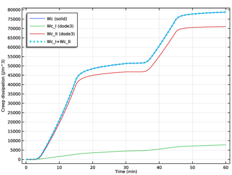
In the associated text field, type Creep dissipation (J/m^3).
5
In the Creep dissipation history toolbar, click  Plot.
Add Physics
1
In the Home toolbar, click  Add Physics to open the Add Physics window.
2
Go to the Add Physics window.
3
In the tree, select Structural Mechanics>Fatigue (ftg).
4
Find the Physics interfaces in study subsection. In the table, clear the Solve check box for Study 1.
5
Click Add to Component 1 in the window toolbar.
Fatigue (ftg)
Strain-Life 1
1
Right-click Component 1 (comp1)>Fatigue (ftg) and choose the domain evaluation Strain-Life.
2
3
In the Settings window for Strain-Life, locate the Fatigue Model Selection section.
4
From the Criterion list, choose Coffin-Manson.
5
From the Strain type list, choose User defined.
6
In the εi text field, type 2*ecxy_II.
7
Locate the Fatigue Model Parameters section. From the εf list, choose User defined. In the associated text field, type 0.587.
8
From the c list, choose User defined. In the associated text field, type -0.61.
Add Physics
1
Go to the Add Physics window.
2
In the tree, select Recently Used>Fatigue (ftg).
3
Find the Physics interfaces in study subsection. In the table, clear the Solve check box for Study 1.
4
Click Add to Component 1 in the window toolbar.
5
In the Physics toolbar, click  Add Physics to close the Add Physics window.
Fatigue 2 (ftg2)
Select Domain 2 only.
Energy-Based 1
1
Right-click Component 1 (comp1)>Fatigue 2 (ftg2) and choose the domain evaluation Energy-Based.
2
3
In the Settings window for Energy-Based, locate the Fatigue Model Selection section.
4
From the Energy type list, choose User defined.
5
In the Wd text field, type Wc_II.
6
Locate the Fatigue Model Parameters section. From the Wf list, choose User defined. In the associated text field, type 74e6.
7
From the m list, choose User defined. In the associated text field, type -0.79.
Add Study
1
In the Home toolbar, click  Add Study to open the Add Study window.
2
Go to the Add Study window.
3
Find the Physics interfaces in study subsection. In the table, clear the Solve check boxes for Solid Mechanics (solid), Domain ODEs and DAEs (dode), Domain ODEs and DAEs 2 (dode2), and Domain ODEs and DAEs 3 (dode3).
4
Find the Studies subsection. In the Select Study tree, select Preset Studies for Selected Physics Interfaces>Fatigue.
5
Click Add Study in the window toolbar.
6
In the Home toolbar, click  Add Study to close the Add Study window.
Study 2
Step 1: Fatigue
1
In the Settings window for Fatigue, locate the Values of Dependent Variables section.
2
Find the Values of variables not solved for subsection. From the Settings list, choose User controlled.
3
From the Method list, choose Solution.
4
From the Study list, choose Study 1, Time Dependent.
5
In the Home toolbar, click  Compute.
The plots shown in Figure 6 and Figure 7 are generated by default.
Results
Max/Min Surface 1
1
In the Model Builder window, expand the Cycles to Failure (ftg) node, then click Max/Min Surface 1.
2
In the Settings window for Max/Min Surface, locate the Coloring and Style section.
3
From the Anchor point list, choose Lower left.
4
In the Cycles to Failure (ftg) toolbar, click  Plot.
Max/Min Surface 1
1
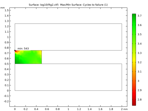
In the Model Builder window, expand the Results>Cycles to Failure (ftg2) node, then click Max/Min Surface 1.
2
In the Settings window for Max/Min Surface, locate the Coloring and Style section.
3
From the Anchor point list, choose Lower left.
4
In the Cycles to Failure (ftg2) toolbar, click  Plot.