PDF

Fountain Flow Effects on Electrodeposition on a Rotating Wafer
Introduction
This example extends the analysis made in the model Electrodeposition on a Resistive Patterned Wafer by including the diffusion and convection of copper ions in the electrolyte.
The coupled mass transport convection-diffusion effects are of interest in this type of reactor since they are accentuated toward the rim of the wafer, limiting the current density. This counterbalances the activation overpotential, which is highest at the rim due to electric current conduction effects in the wafer. By the design of the reactor, the relation between mass transport and activation potential effects can be optimized to make the current distribution over the wafer more uniform.
Note: This application requires the CFD Module.
Model Definition
Due to symmetry the model geometry is made axisymmetrical in two dimensions. The model geometry is shown in Figure 1. A wafer is mounted in a holder of isolating material at the top of the cell and rotates at a given rotational speed of 30 rpm. Electrolyte enters the reactor (which does not rotate) from the bottom at a given flow rate and exits through the narrow gap at the top right in the figure. Copper is deposited on the rotating cathode wafer at a known average current density.
Figure 1: Model geometry, axisymmetrical around r = 0. Two domains are used, with the copper concentration being solved for in the top domain only to save computational time.
Choice of physics
Use the Electrode, Shell physics for solving for the potential on the wafer boundary, (V).
In the cell, use a supporting electrolyte so that the electrolyte conductivity is not affected by local copper concentration changes. This implies that the Secondary Current Distribution physics can be used to model the electrolyte potential (V), and the Transport of Diluted Species physics to model the mass transfer, solving for the electrolyte concentration of copper ions, c (mol/m3).
The relatively low rotational speed, in combination with the large wafer size, implies that the flow is not turbulent. This means that a Laminar Flow interface is suitable for solving for the velocity, v (m/s), and pressure p (Pa).
Electrode, Shell
Use a resistivity of 1.7·106 (Ω·cm) and an electrode layer thickness of either 75 nm or 150 nm. The latter parameter will be varied by the Continuation settings in the solver. Ground the right endpoint of the wafer. Use a Normal Current Density feature to create a current source, which becomes coupled to the Electrode Reaction current density set up by the Secondary Current Distribution physics.
Secondary Current Distribution
Use an electrolyte conductivity of 0.5 (S/m). Set the total current at the inlet boundary to correspond to an average wafer current density (0.5 or 2 A/dm2), which is varied by the Continuation settings in the solver.
On the wafer boundary, use an Electrode Surface node to set up the electrode current density according to
(1)
where i0 (10 A/m2) is the exchange current density, F is Faraday’s constant (96485 C/mol), R is the molar gas constant (8.3145 J/(mol·K)), T is the temperature (298.15 K), and cb (0.3 mol/l) is the bulk concentration of copper ions.
The overpotential, η (V), is defined as
Laminar Flow
Enable Swirl Flow to solve also for the velocity in the  direction. Specify the inflow velocity to correspond to a total flow of 30 l/min, and set the outlet pressure to 0 Pa. Use a Wall boundary condition, with the Sliding Wall feature enabled, to define a rotational velocity for the rotating wafer and the holder boundaries.
Transport of Diluted Species
Since concentration gradients are expected only in the vicinity of the electrode surface, the computational time can be reduced by modeling the copper ion transport in upper domain only.
Use a diffusion coefficient of 5·106 (cm2/s) and couple the convective flow to the velocity solved for by the Laminar Flow physics. Enable Migration and couple it to the electrolyte potential solved for by Secondary Current Distribution physics.
Set the concentration at the inlet boundary to cb and set zero diffusional flux at the outlet using an Outlet condition.
Couple the flux of copper ions at the wafer to the electrode current density in the Secondary Current Distribution physics boundary using an Electrode-Electrolyte Interface Coupling. This sets up a flux condition using Faraday’s law.
Study
Since the flow profile is not affected by any other physics, solve the model in two steps with Laminar Flow only in the first step, and the other physics in the second step. Use a Study Extension with Continuation in the second study step to solve for two different average wafer current densities (0.5 and 2 A/dm2) and two different wafer seed layer thicknesses (75 and 150 nm).
Results and Discussion
Figure 2 shows the concentration in copper ions in the electrolyte. The concentration is lowest toward the rim of the rotating wafer.
Figure 2: Copper concentration for an average wafer current of 200 A/m2 and a seed layer thickness of 150 nm.
Figure 3 shows the velocity steam lines in the reactor. The velocity magnitude is highest close to the rotating surfaces, as indicated by the higher density of streamlines.
Figure 3: Velocity streamlines.
Figure 4 shows the electrode current density as described by Equation 1. The cathodic current density increases toward the rim of the wafer until concentration effects start to dominate, at the end of the wafer the current density drops significantly.
Figure 4: Cathode current density versus radial coordinate.
Notes About the COMSOL Implementation
Use second-order elements in all physics interfaces.
Application Library path: Electrodeposition_Module/Tutorials/fountain_flow
Modeling Instructions
From the File menu, choose New.
New
In the New window, click  Model Wizard.
Model Wizard
1
In the Model Wizard window, click  2D Axisymmetric.
Add the four different physics that are used in this model.
2
In the Select Physics tree, select Chemical Species Transport>Transport of Diluted Species (tds).
3
Click Add.
4
In the Select Physics tree, select Electrochemistry>Primary and Secondary Current Distribution>Secondary Current Distribution (cd).
5
Click Add.
6
In the Select Physics tree, select Electrochemistry>Electrode, Shell (els).
7
Click Add.
8
In the Electric potential text field, type phis_wafer.
9
In the Select Physics tree, select Fluid Flow>Single-Phase Flow>Laminar Flow (spf).
10
Click Add.
11
Click  Study.
12
In the Select Study tree, select General Studies>Stationary.
13
Global Definitions
Parameters 1
Load the model parameters from a text file.
1
In the Model Builder window, under Global Definitions click Parameters 1.
2
In the Settings window for Parameters, locate the Parameters section.
3
Click  Load from File.
4
Geometry 1
Draw the geometry as the union of two rectangles, split one boundary by adding a point. The lower part of the split boundary will become the outlet.
Rectangle 1 (r1)
1
In the Geometry toolbar, click  Rectangle.
2
In the Settings window for Rectangle, locate the Size and Shape section.
3
In the Width text field, type d_cell/2.
4
In the Height text field, type h_cell.
5
Locate the Position section. In the z text field, type -h_cell.
Rectangle 2 (r2)
1
In the Geometry toolbar, click  Rectangle.
2
In the Settings window for Rectangle, locate the Size and Shape section.
3
In the Width text field, type d_wafer/2.
4
In the Height text field, type h_gap.
Point 1 (pt1)
1
In the Geometry toolbar, click  Point.
2
In the Settings window for Point, locate the Point section.
3
In the r text field, type d_wafer/2.
4
In the z text field, type h_outlet.
5
Click  Build All Objects.
6
Click the  Zoom Extents button in the Graphics toolbar.
The finalized geometry should now look like the figure below:
Definitions
Add some explicit selections to facilitate boundary selection when setting up the physics.
Cathode
1
In the Definitions toolbar, click  Explicit.
2
In the Settings window for Explicit, locate the Input Entities section.
3
From the Geometric entity level list, choose Boundary.
4
5
Right-click Explicit 1 and choose Rename.
6
In the Rename Explicit dialog box, type Cathode in the New label text field.
7
Inlet
1
In the Definitions toolbar, click  Explicit.
2
In the Settings window for Explicit, locate the Input Entities section.
3
From the Geometric entity level list, choose Boundary.
4
5
Right-click Explicit 2 and choose Rename.
6
In the Rename Explicit dialog box, type Inlet in the New label text field.
7
Outlet
1
In the Definitions toolbar, click  Explicit.
2
In the Settings window for Explicit, locate the Input Entities section.
3
From the Geometric entity level list, choose Boundary.
4
5
Right-click Explicit 3 and choose Rename.
6
In the Rename Explicit dialog box, type Outlet in the New label text field.
7
Rotating wall
1
In the Definitions toolbar, click  Explicit.
2
In the Settings window for Explicit, locate the Input Entities section.
3
From the Geometric entity level list, choose Boundary.
4
5
Right-click Explicit 4 and choose Rename.
6
In the Rename Explicit dialog box, type Rotating wall in the New label text field.
7
Laminar Flow (spf)
Now start defining the Laminar flow settings of the physics. Enable Swirl Flow to also solve for the velocity in the ϕ direction.
1
In the Settings window for Laminar Flow, locate the Physical Model section.
2
Select the Swirl flow check box.
Fluid Properties 1
1
In the Model Builder window, under Component 1 (comp1)>Laminar Flow (spf) click Fluid Properties 1.
2
In the Settings window for Fluid Properties, locate the Fluid Properties section.
3
From the ρ list, choose User defined. In the associated text field, type rho.
4
From the μ list, choose User defined. In the associated text field, type mu.
Inlet 1
1
In the Physics toolbar, click  Boundaries and choose Inlet.
2
In the Settings window for Inlet, locate the Boundary Selection section.
3
From the Selection list, choose Inlet.
4
Locate the Velocity section. In the U0 text field, type v_in.
Outlet 1
1
In the Physics toolbar, click  Boundaries and choose Outlet.
2
In the Settings window for Outlet, locate the Boundary Selection section.
3
From the Selection list, choose Outlet.
Wall 2
Use a sliding wall to define the rotating surfaces. The velocity is zero in the rz-plane and ωr in the ϕ direction.
1
In the Physics toolbar, click  Boundaries and choose Wall.
2
3
In the Settings window for Wall, click to expand the Wall Movement section.
4
Select the Sliding wall check box.
5
In the vw text field, type omega*r.
Initial Values 1
1
In the Model Builder window, click Initial Values 1.
2
In the Settings window for Initial Values, locate the Initial Values section.
3
Specify the u vector as
4
In the p text field, type 1.
Secondary Current Distribution (cd)
Electrolyte 1
Now set up the model for the electrolyte currents. Start with the electrolyte conductivity.
1
In the Model Builder window, under Component 1 (comp1)>Secondary Current Distribution (cd) click Electrolyte 1.
2
In the Settings window for Electrolyte, locate the Electrolyte section.
3
From the σl list, choose User defined. In the associated text field, type sigma.
Electrode Surface 1
1
In the Physics toolbar, click  Boundaries and choose Electrode Surface.
Set the electric potential of the electrode surface to the potential solved for by the Electrode, Shell physics.
2
In the Settings window for Electrode Surface, locate the Boundary Selection section.
3
From the Selection list, choose Cathode.
4
Locate the Electrode Phase Potential Condition section. In the φs,ext text field, type phis_wafer.
Electrode Reaction 1
Set the electrode kinetics to be dependent on the local concentration of copper ions.
1
In the Model Builder window, expand the Electrode Surface 1 node, then click Electrode Reaction 1.
2
In the Settings window for Electrode Reaction, locate the Equilibrium Potential section.
3
From the Eeq list, choose Nernst equation.
4
In the CO text field, type c/c_bulk.
5
Locate the Stoichiometric Coefficients section. In the n text field, type 2.
6
Locate the Electrode Kinetics section. From the Kinetics expression type list, choose Butler-Volmer.
7
From the Exchange current density type list, choose From Nernst Equation.
8
In the i0,ref(T) text field, type i0.
9
In the αa text field, type 1.5.
Electrolyte Current 1
Define the total current of the cell on the bottom electrolyte boundary.
1
In the Physics toolbar, click  Boundaries and choose Electrolyte Current.
2
In the Settings window for Electrolyte Current, locate the Boundary Selection section.
3
From the Selection list, choose Inlet.
4
Locate the Electrolyte Current section. In the Il,total text field, type I_tot.
Transport of Diluted Species (tds)
Now define the physics for the transport of copper ions. To save computational time, model only the domain in direct vicinity to the electrode surface.
1
In the Model Builder window, under Component 1 (comp1) click Transport of Diluted Species (tds).
2
In the Settings window for Transport of Diluted Species, locate the Domain Selection section.
3
Click  Clear Selection.
4
5
Locate the Transport Mechanisms section. Select the Migration in electric field check box.
Transport Properties 1
1
In the Model Builder window, under Component 1 (comp1)>Transport of Diluted Species (tds) click Transport Properties 1.
2
In the Settings window for Transport Properties, locate the Migration in Electric Field section.
3
In the V text field, type phil.
4
Locate the Diffusion section. In the Dc text field, type D_Cu.
5
Locate the Migration in Electric Field section. In the zc text field, type 2.
The velocity field will be coupled to Laminar Flow later using the Reacting Flow multiphysics feature.
Initial Values 1
1
In the Model Builder window, click Initial Values 1.
2
In the Settings window for Initial Values, locate the Initial Values section.
3
In the c text field, type c_bulk.
Inflow 1
1
In the Physics toolbar, click  Boundaries and choose Inflow.
2
3
In the Settings window for Inflow, locate the Concentration section.
4
In the c0,c text field, type c_bulk.
Outflow 1
1
In the Physics toolbar, click  Boundaries and choose Outflow.
2
In the Settings window for Outflow, locate the Boundary Selection section.
3
From the Selection list, choose Outlet.
Electrode Surface Coupling 1
Define the flux of copper ions on the electrode surface by coupling it to the electrode currents.
1
In the Physics toolbar, click  Boundaries and choose Electrode Surface Coupling.
2
In the Settings window for Electrode Surface Coupling, locate the Boundary Selection section.
3
From the Selection list, choose Cathode.
Reaction Coefficients 1
1
In the Model Builder window, expand the Electrode Surface Coupling 1 node, then click Reaction Coefficients 1.
2
In the Settings window for Reaction Coefficients, locate the Model Inputs section.
3
From the iloc list, choose Local current density, Electrode Reaction 1 (cd/es1/er1).
4
Locate the Stoichiometric Coefficients section. In the n text field, type 2.
5
In the νc text field, type -1.
Electrode, Shell (els)
Now set up the model for the electric potential in the wafer.
1
In the Model Builder window, under Component 1 (comp1) click Electrode, Shell (els).
2
In the Settings window for Electrode, Shell, locate the Boundary Selection section.
3
From the Selection list, choose Cathode.
Electrode 1
1
In the Model Builder window, under Component 1 (comp1)>Electrode, Shell (els) click Electrode 1.
2
In the Settings window for Electrode, locate the Electrode section.
3
In the s text field, type t_seed.
4
From the σ list, choose User defined. In the associated text field, type 1/r_seed.
Ground 1
1
In the Physics toolbar, click  Points and choose Ground.
2
Normal Current Density 1
Couple the wafer potential model to the electrode reaction by adding a current source corresponding to the electrode reaction.
1
In the Physics toolbar, click  Boundaries and choose Normal Current Density.
2
In the Settings window for Normal Current Density, locate the Boundary Selection section.
3
From the Selection list, choose Cathode.
4
Locate the Normal Current Density section. From the in list, choose Local current density, Electrode Reaction 1 (cd/es1/er1).
Multiphysics
Finally, set up the Reactive Flow multiphysics feature.
Reacting Flow, Diluted Species 1 (rfd1)
In the Physics toolbar, click  Multiphysics Couplings and choose Domain>Reacting Flow, Diluted Species.
Mesh 1
Create a triangular mesh with higher resolution close to the electrode surface. Add boundary layers to further improve the accuracy where needed.
Size 1
In the Model Builder window, under Component 1 (comp1) right-click Mesh 1 and choose Size.
Size
1
In the Settings window for Size, locate the Element Size section.
2
From the Calibrate for list, choose Fluid dynamics.
3
From the Predefined list, choose Coarse.
Size 1
1
In the Model Builder window, click Size 1.
2
In the Settings window for Size, locate the Geometric Entity Selection section.
3
From the Geometric entity level list, choose Boundary.
4
From the Selection list, choose Rotating wall.
5
Locate the Element Size section. Click the Custom button.
6
Locate the Element Size Parameters section. Select the Maximum element size check box.
7
Free Triangular 1
In the Mesh toolbar, click  Free Triangular.
Boundary Layers 1
In the Mesh toolbar, click  Boundary Layers.
Boundary Layer Properties
1
In the Model Builder window, click Boundary Layer Properties.
2
3
In the Settings window for Boundary Layer Properties, locate the Boundary Layer Properties section.
4
In the Number of boundary layers text field, type 5.
5
In the Thickness adjustment factor text field, type 5.
6
In the Model Builder window, right-click Mesh 1 and choose Build All.
The finalized mesh should look like this:
Transport of Diluted Species (tds)
Use 2nd-order elements in all interfaces (Electrode, Shell uses 2nd-order elements by default).
1
In the Model Builder window, under Component 1 (comp1) click Transport of Diluted Species (tds).
2
In the Settings window for Transport of Diluted Species, click to expand the Discretization section.
3
From the Concentration list, choose Quadratic.
Secondary Current Distribution (cd)
1
In the Model Builder window, under Component 1 (comp1) click Secondary Current Distribution (cd).
2
In the Settings window for Secondary Current Distribution, click to expand the Discretization section.
3
From the Electrolyte potential list, choose Quadratic.
Laminar Flow (spf)
1
In the Model Builder window, under Component 1 (comp1) click Laminar Flow (spf).
2
In the Settings window for Laminar Flow, click to expand the Discretization section.
3
From the Discretization of fluids list, choose P2+P1.
Study 1
Step 1: Stationary
1
In the Model Builder window, under Study 1 click Step 1: Stationary.
2
In the Settings window for Stationary, locate the Physics and Variables Selection section.
3
In the table, clear the Solve for check boxes for Transport of Diluted Species (tds), Secondary Current Distribution (cd), and Electrode, Shell (els).
Stationary 2
1
In the Study toolbar, click  Study Steps and choose Stationary>Stationary.
2
In the Settings window for Stationary, locate the Physics and Variables Selection section.
3
In the table, clear the Solve for check box for Laminar Flow (spf).
4
Click to expand the Study Extensions section. Select the Auxiliary sweep check box.
5
From the Sweep type list, choose All combinations.
6
7
8
9
In the Study toolbar, click  Compute.
Results
Velocity Streamline
Create a streamline plot of the velocity field in the following way.
1
In the Home toolbar, click  Add Plot Group and choose 2D Plot Group.
2
In the Settings window for 2D Plot Group, type Velocity Streamline in the Label text field.
Streamline 1
1
Right-click Velocity Streamline and choose Streamline.
2
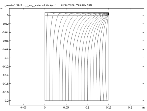
In the Settings window for Streamline, click Replace Expression in the upper-right corner of the Expression section. From the menu, choose Component 1 (comp1)>Laminar Flow>Velocity and pressure>u,w - Velocity field.
3
4
In the Velocity Streamline toolbar, click  Plot.
Local Current Density
Create a line plot of the local electrode current density in the following way.
1
In the Home toolbar, click  Add Plot Group and choose 1D Plot Group.
2
In the Settings window for 1D Plot Group, type Local Current Density in the Label text field.
Line Graph 1
1
Right-click Local Current Density and choose Line Graph.
2
In the Settings window for Line Graph, locate the Selection section.
3
From the Selection list, choose Cathode.
4
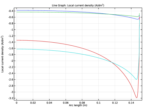
Click Replace Expression in the upper-right corner of the y-Axis Data section. From the menu, choose Component 1 (comp1)>Secondary Current Distribution>Electrode kinetics>cd.iloc_er1 - Local current density - A/m².
5
Locate the y-Axis Data section. In the Unit field, type A/dm^2.
6
In the Local Current Density toolbar, click  Plot.