PDF

Decorative Plating
Introduction
This tutorial example of decorative electroplating models a secondary current distribution with full Butler-Volmer kinetics for both anode and cathode. The thickness of the deposited layer at the cathode is computed along with the surface thickness change on the anode caused by metal dissolution.
A more detailed description of how to build this model, including screenshots, can be found in the Introduction to the Electrodeposition Module book.
Model Definition
The model geometry is shown in Figure 1. The anode is a planar dissolving anode. The cathode represents a furniture fitting that is to be decorated by metal plating.
Figure 1: The model geometry.
The conductivity of the metal of the anode and cathode is very high compared to that of the electrolyte and it is thus assumed that the electric potential in the metal is constant. Variations in the activation overpotential are therefore caused by the potential in the electrolyte at the surface of the electrodes. Under these assumptions, the electrodes are treated as boundaries in the simulations.
Before beginning, one difficulty found in all current density distribution models needs to be discussed. The overpotential, , for an electrode reaction of index m, is defined according to the following equation:
where denotes the electric potential of the metal, denotes the potential in the electrolyte, and Eeq,m denotes the difference between the metal and electrolyte potentials at the electrode surface, measured at equilibrium using a common reference potential. The electric potential of one of the electrodes may be bootstrapped, so that all other potentials are measured with this reference (this bootstrap can actually be achieved by fixing the potential at any point in the cell). In this case, the electric potential of the metal is selected at the cathode as a bootstrap by setting this potential to 0 V. This implies that the electric potential of the metal at the anode is equal to the cell voltage. The potential of the electrolyte floats and adapts to satisfy the balance of current, so that an equal amount of current that leaves at the cathode also enters at the anode. This then determines the overpotential at the anode and the cathode.
Electrolyte charge transport
Use the Secondary Current Distribution interface to solve for the electrolyte potential, φl (SI unit: V), according to:
where il (SI unit: A/m2) is the electrolyte current density vector and σl (SI unit: S/m) is the electrolyte conductivity, which is assumed to be a constant.
Use the default Insulation condition for all boundaries except the anode and cathode surfaces:
where n is the normal vector, pointing out of the domain.
The main electrode reaction on both the anode and the cathode surfaces is the nickel deposition/dissolution reaction according to
Use a Butler-Volmer Expression to model this reaction; this sets the local current density to
The rate of deposition at the cathode boundary surfaces and the rate of dissolution at the anode boundary surface, with a velocity in the normal direction, v (m/s), is calculated according to
where M is the mean molar mass (59 g/mol) and ρ is the density (8900 kg/m3) of the nickel atoms and n is number of participating electrons. Note that the local current density is positive at the anode surface and negative at the cathode surfaces.
On the anode the electrolyte current density is set to the local current density of the nickel deposition reaction:
On the cathode, add a second electrode reaction to model the parasitic hydrogen evolution reaction:
Use a cathodic Tafel equation to model the kinetics of the hydrogen reaction on the cathode, this sets the local current density to
The hydrogen reaction does not contribute to the rate of deposition of nickel, but it contributes to the total current density at the cathode surface:
Solve the model in a time-dependent study, simulating the electroplating for 600 s.
Results and Discussion
Figure 2 shows the change in the total electrode thickness for the cathode surfaces indicating the deposition thickness after 600 s. It can be seen that the deposition thickness is quite non-uniform. The lowest deposition thickness is found at the bottom end of the cathode geometry, farthest from the anode surface. The deposition thickness could be optimized further by changing design parameters such as plating cell geometry, distance between the anode and cathode surface, conductivity of the electrolyte and operational parameters such as applied current or potential.
Figure 2: The simulated results of the change in the total electrode thickness.
Figure 3 shows the local current efficiency over the cathode surface. The efficiency is calculated as the nickel deposition current density divided by the total current density at the cathode. The efficiency is about 97%.
Figure 3: The current efficiency factor at the cathode.
Application Library path: Electrodeposition_Module/Tutorials/decorative_plating
Modeling Instructions
From the File menu, choose New.
New
In the New window, click  Model Wizard.
Model Wizard
1
In the Model Wizard window, click  3D.
2
In the Select Physics tree, select Electrochemistry>Primary and Secondary Current Distribution>Secondary Current Distribution (cd).
3
Click Add.
4
Click  Study.
5
In the Select Study tree, select Preset Studies for Selected Physics Interfaces>Time Dependent with Initialization.
6
Global Definitions
Load the model parameters from a text file.
Parameters 1
1
In the Model Builder window, under Global Definitions click Parameters 1.
2
In the Settings window for Parameters, locate the Parameters section.
3
Click  Load from File.
4
Geometry 1
The model geometry is available as a parameterized geometry sequence in a separate MPH-file. If you want to build it from scratch, follow the instructions in the section Appendix — Geometry Modeling Instructions. Otherwise load it from file with the following steps.
1
In the Geometry toolbar, click  Insert Sequence.
2
3
In the Geometry toolbar, click  Build All.
4
Click the  Wireframe Rendering button in the Graphics toolbar.
5
In the Model Builder window, under Component 1 (comp1) right-click Geometry 1 and choose Plot.
6
Click the  Zoom Extents button in the Graphics toolbar.
Secondary Current Distribution (cd)
Now start setting up the current distribution model, beginning with the settings for the electrolyte.
Electrolyte 1
1
In the Model Builder window, under Component 1 (comp1)>Secondary Current Distribution (cd) click Electrolyte 1.
2
In the Settings window for Electrolyte, locate the Electrolyte section.
3
From the σl list, choose User defined. In the associated text field, type kappa.
Electrode Surface 1
Now define the anode and the nickel dissolution-deposition electrode reaction on this surface. The combination of the properties of the surface and the reaction stoichiometry will determine how the magnitude and direction of the growth velocity of the deposited layer relates to the electrode reaction currents.
1
In the Physics toolbar, click  Boundaries and choose Electrode Surface.
2
Keep the default boundary condition for this surface, setting the electric potential to zero (grounding the electrode).
3
In the Settings window for Electrode Surface, click to expand the Dissolving-Depositing Species section.
4
5
Electrode Reaction 1
Set the first electrode reaction to be the nickel deposition reaction.
1
In the Model Builder window, expand the Electrode Surface 1 node, then click Electrode Reaction 1.
2
In the Settings window for Electrode Reaction, locate the Stoichiometric Coefficients section.
3
In the n text field, type 2.
4
In the Stoichiometric coefficients for dissolving-depositing species: table, enter the following settings:
5
Locate the Equilibrium Potential section. In the Eeq text field, type Eeq_Ni.
6
Locate the Electrode Kinetics section. From the Kinetics expression type list, choose Butler-Volmer.
7
In the i0 text field, type i0_Ni.
Electrode Surface 1
Now duplicate this node to define the cathode.
Electrode Surface 2
1
In the Model Builder window, under Component 1 (comp1)>Secondary Current Distribution (cd) right-click Electrode Surface 1 and choose Duplicate.
2
In the Settings window for Electrode Surface, locate the Boundary Selection section.
3
From the Selection list, choose Cathode.
4
Locate the Electrode Phase Potential Condition section. From the Electrode phase potential condition list, choose Average current density.
5
In the il,average text field, type Iavg.
6
In the Model Builder window, expand the Electrode Surface 2 node.
Electrode Reaction 1
1
In the Model Builder window, expand the Electrode Surface 2 node, then click Electrode Reaction 1.
2
In the Settings window for Electrode Reaction, locate the Stoichiometric Coefficients section.
3
In the Stoichiometric coefficients for dissolving-depositing species: table, enter the following settings:
Electrode Surface 2
Add the hydrogen evolution reaction.
In the Model Builder window, click Electrode Surface 2.
Electrode Reaction 2
1
In the Physics toolbar, click  Attributes and choose Electrode Reaction.
2
In the Settings window for Electrode Reaction, locate the Electrode Kinetics section.
3
From the Kinetics expression type list, choose Cathodic Tafel equation.
4
In the i0 text field, type i0_H.
Mesh 1
1
In the Model Builder window, under Component 1 (comp1) click Mesh 1.
2
In the Settings window for Mesh, locate the Physics-Controlled Mesh section.
3
From the Element size list, choose Finer.
4
Click  Build All.
5
Right-click Component 1 (comp1)>Mesh 1 and choose Plot.
6
Click the  Zoom Extents button in the Graphics toolbar.
Study 1
Step 1: Current Distribution Initialization
1
In the Model Builder window, under Study 1 click Step 1: Current Distribution Initialization.
2
In the Settings window for Current Distribution Initialization, locate the Study Settings section.
3
From the Current distribution type list, choose Secondary.
Step 2: Time Dependent
1
In the Model Builder window, click Step 2: Time Dependent.
2
In the Settings window for Time Dependent, locate the Study Settings section.
3
In the Output times text field, type range(0,60,600).
4
In the Home toolbar, click  Compute.
Results
Deposited Thickness, Cathode
Modify the default plot for the electrode thickness change to show the deposited thickness on the cathode only.
1
In the Model Builder window, click Total Electrode Thickness Change (cd).
2
In the Settings window for 3D Plot Group, click to expand the Selection section.
3
From the Geometric entity level list, choose Boundary.
4
From the Selection list, choose Cathode.
5
In the Total Electrode Thickness Change (cd) toolbar, click  Plot.
6
Click the  Zoom Extents button in the Graphics toolbar.
7
Right-click Total Electrode Thickness Change (cd) and choose Rename.
8
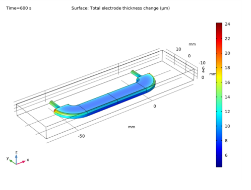
In the Rename 3D Plot Group dialog box, type Deposited Thickness, Cathode in the New label text field.
9
Deposited Thickness, Cathode 1
Right-click Deposited Thickness, Cathode and choose Duplicate.
Surface 1
1
In the Model Builder window, expand the Deposited Thickness, Cathode 1 node, then click Surface 1.
2
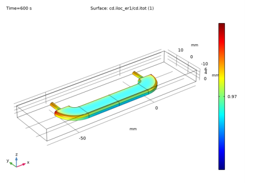
In the Settings window for Surface, click Replace Expression in the upper-right corner of the Expression section. From the menu, choose Component 1 (comp1)>Secondary Current Distribution>Electrode kinetics>cd.iloc_er1 - Local current density - A/m².
Divide the current density of the nickel reaction with the total current density variable.
3
Locate the Expression section. In the Expression text field, type cd.iloc_er1/cd.itot.
4
In the Deposited Thickness, Cathode 1 toolbar, click  Plot.
5
Click the  Zoom Extents button in the Graphics toolbar.
Current Efficiency, Cathode
1
In the Model Builder window, right-click Deposited Thickness, Cathode 1 and choose Rename.
2
In the Rename 3D Plot Group dialog box, type Current Efficiency, Cathode in the New label text field.
3
Appendix — Geometry Modeling Instructions
Add Component
1
In the Model Builder window, expand the Results node.
2
Definitions
In the Model Builder window, expand the Component 1 (comp1)>Definitions node.
View 1
1
In the Model Builder window, expand the Component 1 (comp1)>Definitions>View 1 node, then click View 1.
2
In the Settings window for View, locate the View section.
3
Select the Wireframe rendering check box.
Geometry 1
1
In the Model Builder window, under Component 1 (comp1) click Geometry 1.
2
In the Settings window for Geometry, locate the Units section.
3
From the Length unit list, choose mm.
Block 1 (blk1)
1
In the Geometry toolbar, click  Block.
2
In the Settings window for Block, locate the Size and Shape section.
3
In the Width text field, type 100.
4
In the Depth text field, type 28.
5
In the Height text field, type 7.25.
6
Locate the Position section. In the x text field, type -70.
7
In the y text field, type -10.
8
In the z text field, type -1.25.
9
Locate the Selections of Resulting Entities section. Select the Resulting objects selection check box.
Cylinder 1 (cyl1)
1
In the Geometry toolbar, click  Cylinder.
2
In the Settings window for Cylinder, locate the Size and Shape section.
3
In the Radius text field, type 1.25.
4
In the Height text field, type 10.
5
Locate the Position section. In the x text field, type -48.
6
In the y text field, type 8.
7
In the z text field, type -1.25.
8
Locate the Axis section. From the Axis type list, choose y-axis.
Cumulative Selections
In the Geometry toolbar, click  Selections and choose Cumulative Selections.
Objects to subtract
1
Right-click Cumulative Selections and choose Cumulative Selection.
2
In the Settings window for Selection, type Objects to subtract in the Label text field.
Cylinder 1 (cyl1)
1
In the Model Builder window, click Cylinder 1 (cyl1).
2
In the Settings window for Cylinder, locate the Selections of Resulting Entities section.
3
Find the Cumulative selection subsection. From the Contribute to list, choose Objects to subtract.
Work Plane 1 (wp1)
1
In the Geometry toolbar, click  Work Plane.
2
In the Settings window for Work Plane, locate the Plane Definition section.
3
From the Plane list, choose zx-plane.
4
In the y-coordinate text field, type 8.
Work Plane 1 (wp1)>Plane Geometry
In the Model Builder window, click Plane Geometry.
Work Plane 1 (wp1)>Rectangle 1 (r1)
1
In the Work Plane toolbar, click  Rectangle.
2
In the Settings window for Rectangle, locate the Size and Shape section.
3
In the Width text field, type 2.5.
4
In the Height text field, type 10.
5
Locate the Position section. In the xw text field, type -1.25.
6
In the yw text field, type -53.
Work Plane 1 (wp1)>Fillet 1 (fil1)
1
In the Work Plane toolbar, click  Fillet.
2
On the object r1, select Points 2 and 3 only.
3
In the Settings window for Fillet, locate the Radius section.
4
In the Radius text field, type 1.
View 2
1
In the Model Builder window, expand the Component 1 (comp1)>Geometry 1>Work Plane 1 (wp1)>View 2 node, then click View 2.
2
On the object r1, select Point 3 only.
Work Plane 1 (wp1)>Fillet 1 (fil1)
1
In the Model Builder window, click Fillet 1 (fil1).
2
In the Settings window for Fillet, click  Build Selected.
Revolve 1 (rev1)
1
In the Geometry toolbar, click  Revolve.
2
In the Settings window for Revolve, locate the Revolution Angles section.
3
Clear the Keep original faces check box.
4
Click the Angles button.
5
In the End angle text field, type 90.
6
Locate the Revolution Axis section. From the Axis type list, choose 3D.
7
Find the Point on the revolution axis subsection. In the x text field, type -40.
8
In the y text field, type 8.
9
In the z text field, type -1.25.
10
Find the Direction of revolution axis subsection. In the y text field, type 0.
11
In the z text field, type 1.
12
Locate the Selections of Resulting Entities section. Find the Cumulative selection subsection. From the Contribute to list, choose Objects to subtract.
Extrude 1 (ext1)
1
In the Geometry toolbar, click  Extrude.
2
In the Settings window for Extrude, locate the General section.
3
From the Input objects list, choose Objects to subtract.
4
From the Extrude from list, choose Faces.
5
From the Input faces list, choose Objects to subtract.
6
7
Click  Remove from Selection.
8
On the object cyl1, select Boundaries 1–6 only.
9
On the object rev1, select Boundaries 1–8 only.
10
Click  Remove from Selection.
11
On the object cyl1, select Boundaries 1–6 only.
12
On the object rev1, select Boundaries 1–8 only.
13
In the tree, select cyl1>1 (not applicable), cyl1>2 (not applicable), cyl1>3, cyl1>4, cyl1>5 (not applicable), and cyl1>6 (not applicable).
14
Click  Remove from Selection.
15
On the object rev1, select Boundaries 1–8 only.
16
In the tree, select rev1>1, rev1>2 (not applicable), rev1>3, rev1>4 (not applicable), rev1>5, rev1>6 (not applicable), and rev1>7 (not applicable).
17
Click  Remove from Selection.
18
On the object rev1, select Boundary 8 only.
19
20
Locate the Distances section. In the table, enter the following settings:
21
Locate the Selections of Resulting Entities section. Find the Cumulative selection subsection. From the Contribute to list, choose Objects to subtract.
22
Click  Build Selected.
Mirror 1 (mir1)
1
In the Model Builder window, right-click Geometry 1 and choose Transforms>Mirror.
2
In the Settings window for Mirror, locate the Input section.
3
From the Input objects list, choose Objects to subtract.
4
Select the Keep input objects check box.
5
Locate the Point on Plane of Reflection section. In the x text field, type -20.
6
Locate the Normal Vector to Plane of Reflection section. In the x text field, type 1.
7
In the z text field, type 0.
8
Locate the Selections of Resulting Entities section. Find the Cumulative selection subsection. From the Contribute to list, choose Objects to subtract.
Difference 1 (dif1)
1
In the Geometry toolbar, click  Booleans and Partitions and choose Difference.
2
In the Settings window for Difference, locate the Difference section.
3
From the Objects to add list, choose Block 1.
4
From the Objects to subtract list, choose Objects to subtract.
Cathode
1
In the Geometry toolbar, click  Selections and choose Box Selection.
2
In the Settings window for Box Selection, type Cathode in the Label text field.
3
Locate the Geometric Entity Level section. From the Level list, choose Boundary.
4
Locate the Box Limits section. In the x minimum text field, type -55.
5
In the x maximum text field, type 15.
6
In the y minimum text field, type -8.
7
In the y maximum text field, type 15.
8
In the z minimum text field, type 0.
9
In the z maximum text field, type 4.