PDF

Copper Electroless Deposition
Introduction
In the electroless deposition, partial oxidation and reduction reactions occur simultaneously at the same position at the electrode surface. The difference between the equilibrium potentials for the two reactions is hence the driving force for the deposition process. The potential at the electrode surface is estimated from the mixed potential theory so that the total anode current density is equal and opposite to the total cathode current density (Ref. 1 and Ref. 2). Since the sum of all reaction current densities sum up to zero locally on the surface, the electroless deposition can be used for plating on objects with low electric conductivity, for instance plastics.
This model simulates copper electroless deposition wherein copper reduction is a cathodic reaction and formaldehyde oxidation is an anodic reaction. The model accounts for mass transport by diffusion and electrochemical reactions at the electrode surface. The equilibrium potentials of partial electrochemical reactions are considered to be concentration dependent. The model estimates the change in current density, deposition thickness and concentration of ionic species during the electroless deposition.
Model Definition
The model is solved over a 1D computational domain that consists of a diffusion layer with an electrode surface at one end and a bulk electrolyte at the other end, as shown in Figure 1. The diffusion layer thickness is set to 2 mm.
Figure 1: Description of the boundary layer adjacent to the steel surface.
Mass transport by diffusion for five ionic species is solved using the Electroanalysis physics interface:
(1)
where ci (mol/m3) is the concentration, Ni (mol/(m2·s)) is the flux vector, Di (m2/s) is the diffusion coefficient, and subscript i indicates ith species. All species are assumed to be diluted in water. The species along with their diffusion coefficients and initial concentrations are tabulated in Table 1.
D (m2/s)·109
cref (mol/m3)·10-3
Cu(OH)2L2-4
L-2
Concentration at the bulk electrolyte boundary is set to the reference concentration as tabulated in Table 1.
(2)
At the electrode surface boundary, an Electrode Surface boundary condition is used wherein the total current is set to 0. This boundary condition yields a constant potential, , at the electrode surface boundary, which satisfies the condition:
(3)
where
(4)
The initial value for boundary electric potentials is set to -0.85 V.
Electrochemical reactions
The following electrochemical reactions occur at the electrode surface:
Copper reduction
(5)
Formaldehyde oxidation
(6)
Concentration dependent kinetics is used to model copper reduction and formaldehyde oxidation reactions, which will set the local current density according to
(7)
where i0,m is the exchange current density, CR,m is the reduced species expression, CO,m is the oxidized species expression and η,m is the overpotential for species m (Cu and HCHO, respectively).
The overpotential η,m (V) is calculated from
(8)
The equilibrium potentials for the copper reduction and formaldehyde oxidation reactions are calculated using the Nernst Equation,
(9)
(10)
At the electrode surface boundary, fluxes of ionic species are defined in terms of the electrochemical reactions as
(11)
where is the stoichiometric coefficient, ij is the local current density, nj is the number of electrons and F is Faraday’s constant (96485 C/mol). The subscript j signifies the electrochemical reaction. This will set the flux to be proportional to the electrode current density according to Faraday’s law. The electrode kinetics parameters: i0,Cu=1 A/m2 and i0,HCHO=1 A/m2 are taken from the current-potential curves reported in Ref. 2.
Results and Discussion
Figure 2 shows the change in the mixed potential at the electrode surface during electroless deposition. It can be seen that the change is significant during the initial stages of deposition, which is attributed to the equilibrium potentials of copper reduction and formaldehyde oxidation reactions, and the constraint of equal and opposite anode and cathode current densities. At about 400 s the potential reaches a maximum.
Figure 2: The change in the mixed potential at the electrode surface against time during electroless deposition.
Figure 3 shows the change in the local current density at the electrode surface during electroless deposition. It can be seen that the current density is considerably increased in the initial stages of electroless deposition, corresponding to the trend observed for the mixed potential in Figure 2.
Figure 3: The change in the local current density at the electrode surface against time during electroless deposition.
Figure 4 shows the change in the deposition thickness at the electrode surface during electroless deposition. It can be seen that after approximately 400 s, the increase in electroless plating thickness is almost linear with time.
Figure 4: The change in the deposition thickness at the electrode surface against time during electroless deposition.
Figure 5 shows the change in the normalized concentration of various ionic species at the electrode surface during electroless deposition. It can be seen that the concentrations of the copper complex and formaldehyde species decrease with time, since they are consumed during the deposition. The free tartrate ligand (L22) concentration increases with time since it is produced in the deposition process.
Figure 5: The change in the normalized concentration at the electrode surface against time during electroless deposition.
References
1. M. Ramasubramanian, B.N. Popov, R.E. White, and K.S. Chen, “A Mathematical Model for Electroless Copper Deposition on Planar Substrates”, Journal of The Electrochemical Society, vol. 146, no. 1, pp. 111–116, 1999.
2. M. Paunovich and M. Schlesinger, Fundamentals of electrochemical deposition, 2nd edition, Chapter 8, Wiley-Interscience, a John Wiley & Sons, Inc. Publication, 2006.
Application Library path: Electrodeposition_Module/Tutorials/cu_electroless_deposition
Modeling Instructions
From the File menu, choose New.
New
In the New window, click  Model Wizard.
Model Wizard
1
In the Model Wizard window, click  1D.
2
In the Select Physics tree, select Electrochemistry>Electroanalysis (tcd).
3
Click Add.
4
In the Number of species text field, type 4.
5
In the Concentrations table, enter the following settings:
6
Click  Study.
7
In the Select Study tree, select General Studies>Time Dependent.
8
Global Definitions
Load the model parameters from a text file.
Parameters 1
1
In the Model Builder window, under Global Definitions click Parameters 1.
2
In the Settings window for Parameters, locate the Parameters section.
3
Click  Load from File.
4
Geometry 1
The geometry consists of a single interval.
Interval 1 (i1)
1
In the Model Builder window, under Component 1 (comp1) right-click Geometry 1 and choose Interval.
2
In the Model Builder window, expand the Geometry 1 node, then click Interval 1 (i1).
3
In the Settings window for Interval, locate the Interval section.
4
5
Click  Build All Objects.
Electroanalysis (tcd)
Start defining the physics.
Electrolyte 1
1
In the Model Builder window, under Component 1 (comp1)>Electroanalysis (tcd) click Electrolyte 1.
2
In the Settings window for Electrolyte, locate the Diffusion section.
3
In the DcCuOH2L2 text field, type DCuOH2L2.
4
In the DcHCHO text field, type DHCHO.
5
In the DcOH text field, type DOH.
6
In the DcL text field, type DL.
Initial Values 1
Set the initial values to the bulk equilibrium concentration.
1
In the Model Builder window, click Initial Values 1.
2
In the Settings window for Initial Values, locate the Initial Values section.
3
In the cCuOH2L2 text field, type cCuOH2L20.
4
In the cHCHO text field, type cHCHO0.
5
In the cOH text field, type cOH0.
6
In the cL text field, type cL0.
Concentration 1
Similarly, now set the concentrations at the bulk electrolyte boundary to the equilibrium concentrations.
1
In the Physics toolbar, click  Boundaries and choose Concentration.
2
3
In the Settings window for Concentration, locate the Concentration section.
4
Select the Species cCuOH2L2 check box.
5
In the c0,cCuOH2L2 text field, type cCuOH2L20.
6
Select the Species cHCHO check box.
7
In the c0,cHCHO text field, type cHCHO0.
8
Select the Species cOH check box.
9
In the c0,cOH text field, type cOH0.
10
Select the Species cL check box.
11
In the c0,cL text field, type cL0.
Electrode Surface 1
Now define the electrode surface. Set the total current to zero at the Electrode Surface, define the depositing species properties, and the copper reduction and formaldehyde oxidation electrode reactions.
1
In the Physics toolbar, click  Boundaries and choose Electrode Surface.
2
3
In the Settings window for Electrode Surface, click to expand the Dissolving-Depositing Species section.
4
5
6
Locate the Electrode Phase Potential Condition section. From the Electrode phase potential condition list, choose Total current.
7
In the Il,total text field, type 0.
8
In the φs,ext,init text field, type -0.65[V].
Electrode Reaction 1
1
In the Model Builder window, expand the Electrode Surface 1 node, then click Electrode Reaction 1.
2
In the Settings window for Electrode Reaction, locate the Stoichiometric Coefficients section.
3
In the νcCuOH2L2 text field, type -1/2.
4
In the νcOH text field, type 1.
5
In the νcL text field, type 1.
6
In the Stoichiometric coefficients for dissolving-depositing species: table, enter the following settings:
7
Locate the Equilibrium Potential section. In the Eeq,ref(T) text field, type Eeq0_Cu.
8
Click to expand the Reference Concentrations section. In the table, enter the following settings:
9
Locate the Electrode Kinetics section. In the i0,ref(T) text field, type i0_Cu.
10
In the αa text field, type 1-alphac_Cu.
Electrode Surface 1
In the Model Builder window, click Electrode Surface 1.
Electrode Reaction 2
1
In the Physics toolbar, click  Attributes and choose Electrode Reaction.
2
In the Settings window for Electrode Reaction, locate the Stoichiometric Coefficients section.
3
In the νcHCHO text field, type 1.
4
In the νcOH text field, type 2.
5
Locate the Equilibrium Potential section. From the Eeq list, choose User defined. In the associated text field, type Eeq0_HCHO.
6
Locate the Electrode Kinetics section. From the Kinetics expression type list, choose Anodic Tafel equation.
7
In the i0 text field, type i0_HCHO*(cOH/cOH0)^2*(cHCHO/cHCHO0).
8
In the Aa text field, type Aa_HCHO.
Global Definitions
Default Model Inputs
Set up the temperature value used in the entire model.
1
In the Model Builder window, under Global Definitions click Default Model Inputs.
2
In the Settings window for Default Model Inputs, locate the Browse Model Inputs section.
3
In the tree, select General>Temperature (K) - minput.T.
4
Find the Expression for remaining selection subsection. In the Temperature text field, type T.
Mesh 1
Build a mesh with a finer resolution at the electrode surface.
1
In the Model Builder window, under Component 1 (comp1) click Mesh 1.
2
In the Settings window for Mesh, locate the Physics-Controlled Mesh section.
3
From the Element size list, choose Extremely fine.
Size 1
1
Right-click Component 1 (comp1)>Mesh 1 and choose Size.
2
In the Settings window for Size, locate the Geometric Entity Selection section.
3
From the Geometric entity level list, choose Boundary.
4
5
Locate the Element Size section. Click the Custom button.
6
Locate the Element Size Parameters section. Select the Maximum element size check box.
7
Edge 1
1
In the Mesh toolbar, click  Edge.
2
In the Settings window for Edge, click  Build All.
Study 1
Finally, set the time dependent solver settings and then the model is ready to run.
1
In the Model Builder window, click Study 1.
2
In the Settings window for Study, locate the Study Settings section.
3
Clear the Generate default plots check box.
Step 1: Time Dependent
1
In the Model Builder window, under Study 1 click Step 1: Time Dependent.
2
In the Settings window for Time Dependent, locate the Study Settings section.
3
In the Output times text field, type range(0,10,3600).
4
From the Tolerance list, choose User controlled.
5
In the Relative tolerance text field, type 1e-5.
6
In the Home toolbar, click  Compute.
Results
The following reproduces the plots from the Results and Discussion section. First, plot the change in the mixed potential with time.
Mixed Potential
1
In the Home toolbar, click  Add Plot Group and choose 1D Plot Group.
2
In the Settings window for 1D Plot Group, type Mixed Potential in the Label text field.
Point Graph 1
1
Right-click Mixed Potential and choose Point Graph.
2
3
In the Settings window for Point Graph, locate the y-Axis Data section.
4
In the Expression text field, type tcd.phisext.
5
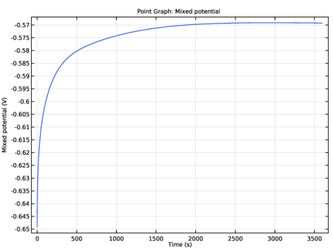
Select the Description check box.
6
7
Click to expand the Title section. From the Title type list, choose Manual.
8
In the Title text area, type Point Graph: Mixed potential.
9
In the Mixed Potential toolbar, click  Plot.
Mixed Potential
Now, plot change in the deposition current density and deposition thickness with time.
Deposition Current Density
1
In the Model Builder window, right-click Mixed Potential and choose Duplicate.
2
In the Settings window for 1D Plot Group, type Deposition Current Density in the Label text field.
Point Graph 1
1
In the Model Builder window, expand the Deposition Current Density node, then click Point Graph 1.
2
In the Settings window for Point Graph, locate the y-Axis Data section.
3
In the Expression text field, type abs(tcd.iloc_er1).
4
In the Description text field, type Deposition current density.
5
Locate the Title section. In the Title text area, type Point Graph: Deposition current density.
6
In the Deposition Current Density toolbar, click  Plot.
Deposition Thickness
1
In the Model Builder window, right-click Mixed Potential and choose Duplicate.
2
In the Model Builder window, click Mixed Potential 1.
3
In the Settings window for 1D Plot Group, type Deposition Thickness in the Label text field.
Point Graph 1
1
In the Model Builder window, click Point Graph 1.
2
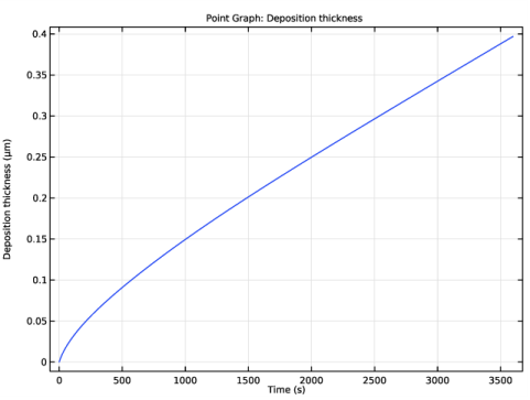
In the Settings window for Point Graph, click Replace Expression in the upper-right corner of the y-Axis Data section. From the menu, choose Component 1 (comp1)>Electroanalysis>Dissolving-depositing species>tcd.sbtot - Total electrode thickness change - m.
3
Locate the y-Axis Data section. From the Unit list, choose µm.
4
In the Description text field, type Deposition thickness.
5
Locate the Title section. In the Title text area, type Point Graph: Deposition thickness.
6
In the Deposition Thickness toolbar, click  Plot.
Mixed Potential
Finally, plot change in the normalized concentration of selected species with time.
Normalized concentration
1
In the Model Builder window, right-click Mixed Potential and choose Duplicate.
2
In the Settings window for 1D Plot Group, type Normalized concentration in the Label text field.
3
Locate the Plot Settings section. Select the y-axis label check box.
4
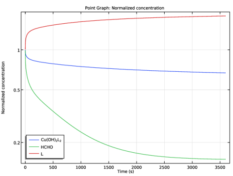
In the associated text field, type Normalized concentration.
5
Locate the Axis section. Select the y-axis log scale check box.
Point Graph 1
1
In the Model Builder window, expand the Normalized concentration node, then click Point Graph 1.
2
In the Settings window for Point Graph, locate the y-Axis Data section.
3
In the Expression text field, type cCuOH2L2/cCuOH2L20.
4
Click to expand the Legends section. Select the Show legends check box.
5
From the Legends list, choose Manual.
6
7
Locate the Title section. In the Title text area, type Point Graph: Normalized concentration.
Point Graph 2
1
Right-click Results>Normalized concentration>Point Graph 1 and choose Duplicate.
2
In the Settings window for Point Graph, locate the y-Axis Data section.
3
In the Expression text field, type cHCHO/cHCHO0.
4
Locate the Legends section. In the table, enter the following settings:
5
Locate the Title section. From the Title type list, choose None.
Point Graph 3
1
Right-click Point Graph 2 and choose Duplicate.
2
In the Settings window for Point Graph, locate the y-Axis Data section.
3
In the Expression text field, type cL/cL0.
4
Locate the Legends section. In the table, enter the following settings:
5
In the Normalized concentration toolbar, click  Plot.
Normalized concentration
1
In the Model Builder window, click Normalized concentration.
2
In the Settings window for 1D Plot Group, locate the Legend section.
3
From the Position list, choose Lower left.