|
|
|
|
1
|
|
2
|
In the Select Physics tree, select Electrochemistry>Primary and Secondary Current Distribution>Secondary Current Distribution (cd).
|
|
3
|
Click Add.
|
|
4
|
Click
|
|
5
|
|
6
|
Click
|
|
1
|
|
2
|
|
3
|
|
4
|
Browse to the model’s Application Libraries folder and double-click the file al_anodization_parameters.txt.
|
|
1
|
|
2
|
|
3
|
|
1
|
|
2
|
|
3
|
|
4
|
|
1
|
|
2
|
|
3
|
|
4
|
|
5
|
|
6
|
|
7
|
|
1
|
|
2
|
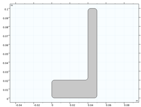
Select the object r1 only.
|
|
3
|
|
4
|
|
5
|
Select the object r2 only.
|
|
6
|
|
1
|
|
2
|
|
3
|
|
4
|
|
5
|
|
1
|
|
2
|
Select the object fil1 only.
|
|
3
|
|
4
|
|
5
|
|
6
|
|
7
|
|
1
|
|
2
|
|
4
|
Locate the Selections of Resulting Entities section. Find the Cumulative selection subsection. Click New.
|
|
5
|
|
6
|
Click OK.
|
|
7
|
|
8
|
|
1
|
|
2
|
|
3
|
|
4
|
|
5
|
|
6
|
|
7
|
|
1
|
|
2
|
|
3
|
|
4
|
|
5
|
|
6
|
|
7
|
|
8
|
|
1
|
|
2
|
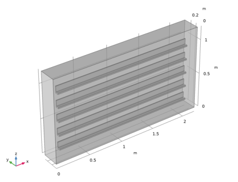
Select the object blk1 only.
|
|
3
|
|
4
|
|
5
|
Select the object mov1 only.
|
|
6
|
|
1
|
In the Model Builder window, under Component 1 (comp1)>Secondary Current Distribution (cd) click Electrolyte 1.
|
|
2
|
|
3
|
|
1
|
|
2
|
|
3
|
|
4
|
Click Browse.
|
|
5
|
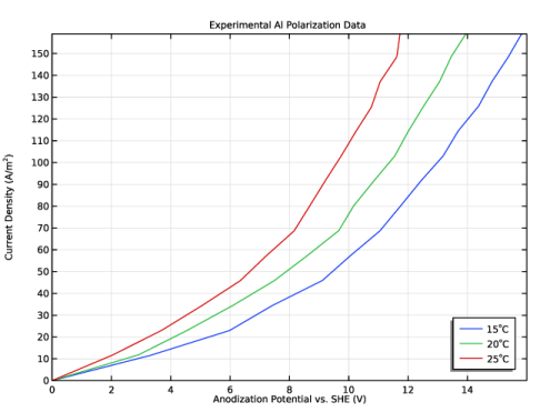
Browse to the model’s Application Libraries folder and double-click the file al_polarization_data.csv.
|
|
6
|
Click Import.
|
|
7
|
Find the Functions subsection. In the table, enter the following settings:
|
|
8
|
|
9
|
|
1
|
|
2
|
|
3
|
|
4
|
|
1
|
|
2
|
|
3
|
|
4
|
Locate the Electrode Phase Potential Condition section. From the Electrode phase potential condition list, choose Average current density.
|
|
5
|
|
6
|
|
1
|
|
2
|
|
3
|
From the iloc,expr list, choose User defined. In the associated text field, type iloc_Al(cd.Evsref,T).
|
|
1
|
|
1
|
|
2
|
|
3
|
|
1
|
In the Model Builder window, under Component 1 (comp1) right-click Mesh 1 and choose Edit Physics-Induced Sequence.
|
|
2
|
|
3
|
|
1
|
|
2
|
|
3
|
|
5
|
|
6
|
|
1
|
|
2
|
|
3
|
|
4
|
Click
|
|
6
|
|
1
|
|
1
|
|
2
|
|
3
|
|
4
|
|
1
|
|
2
|
|
1
|
|
2
|
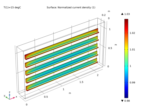
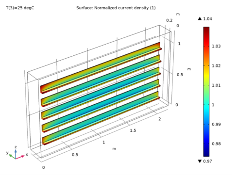
In the Settings window for 3D Plot Group, type Normalized Current Distribution in the Label text field.
|
|
3
|
|
4
|
|
5
|
|
1
|
|
2
|
|
3
|
|
4
|
Select the Description check box.
|
|
5
|
In the associated text field, type Normalized current density.
|
|
6
|
|
1
|
|
2
|
|
3
|
|
4
|
|
5
|
|
6
|
|
7
|
|
8
|
|
1
|
|
2
|
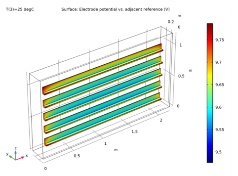
In the Settings window for 3D Plot Group, type Deposited Layer Thickness after 25 min in the Label text field.
|
|
1
|
In the Model Builder window, expand the Deposited Layer Thickness after 25 min node, then click Surface 1.
|
|
2
|
|
3
|
|
4
|
|
5
|
|
6
|