PDF

Wire Electrode
Introduction
One of the most important aspects in the design of electrochemical cells is the current density distributions in the electrolyte and electrodes. Non-uniform current density distributions can be detrimental for the operation of electrochemical processes. In many cases the parts of an electrode that are subjected to high current density degrade at a faster rate. Knowledge of the current density distribution is also desired to optimize the utilization of the electrocatalysts, because these are often made of expensive noble metals. Non-uniform deposition and consumption, as well as unnecessarily high overvoltages, with resulting energy losses and possibly unwanted side-reactions, may be other effects that one would like to minimize.
This example models the primary, secondary, and tertiary current density distributions (Ref. 1) of an arbitrary electrochemical cell. It successively goes through the different classes of current density distributions so as to also show how complexity should be gradually introduced when modeling electrochemical cells.
The same geometry is considered in all three cases: a wire electrode structure is placed between two flat electrode surfaces, and in the open volume between the wire and the flat surfaces electrolyte is allowed to flow; see Figure 1. The electrochemical cell can be seen as a unit cell of a larger wire-mesh electrode — an electrochemical cell setup common for many large-scale industrial processes.
.
Figure 1: Modeled electrochemical cell. Wire electrode (anode) between two flat electrodes (cathodes). Flow inlet to the left, outlet to the right. The top and bottom flat surfaces are inert.
Model Definition
PRIMARY CURRENT DISTRIBUTION
Figure 1 shows the investigated geometry. Firstly, this example considers primary current density distribution. This is the situation where the mixing of electrolyte is vigorous or where concentration gradients are small, so that ionic migration is the dominating transport mechanism. The general mass balance in the electrolyte, assuming steady-state conditions and that no homogeneous reactions occur, can be given by
where Ni is the flux of species i (SI unit: mol·m2/s), which in turn is governed by:
(1)
where ci represents the concentration of the ion i (SI unit: mol/m3), zi its valence, Di its diffusivity (SI unit: m2/s), mi its mobility (SI unit: mol·m2(s·V·A)), F denotes the Faraday constant (SI unit: As/mol), the ionic potential, and u the velocity vector (SI unit: m/s). The components operated upon by the above transport equation are often described as the diffusion, migration, and convection transport mechanisms. The net current density can be described through:
where i is the current density vector (SI unit: A/m2). Combining the three above equations, while assuming electroneutrality (which removes the convection term) and negligible concentration gradients (which removes diffusion) leaves:
Current density is conserved throughout:
(2)
so that by combining the valence, ionic mobility, constant concentration and the Faraday constant to a representative conductivity, κ (SI unit: S/m)), Equation 2 becomes:
(3)
This final equation is equivalent to Ohm’s Law.
The boundary conditions for the case of primary current density distribution assume that the kinetics on the electrode surfaces are fast, which allow the assumption of constant potential on these surfaces (all other boundaries are insulated). The solid phase (electronic conductor) potential on the cathode, (SI unit: V), is a convenient choice of reference potential in the system:
The electrode potential equals the difference between the potential of solid phase in the electrode, , and the potential in the adjacent electrolyte, :
In the absence of kinetic losses, the cathode potential, Ec, equals the equilibrium potential, Eeq,c:
which sets the boundary condition for the cathode.
The potential difference over the whole cell, Ecell, is defined as the potential difference between the solid phases of the two electrodes
In this way the boundary condition for the ionic potential at the anode can be set via:
SECONDARY CURRENT DISTRIBUTION
Secondary current distribution takes into account the kinetics at the electrodes. Mixing is supposed to be good and the electroneutrality condition still relevant so that Ohm’s Law remains a good description for the equations in the domain. Yet the electrochemical reactions are no longer fast enough that a constant potential can be applied at the electrodes. The properties of the chemical species and their ability to react at the surface, that is, the reaction driving forces (overvoltages), need to be considered.
In this model, the expressions for the local current density, i (SI unit: A/m2), is based on the Butler-Volmer equation (Ref. 2) for a single electron reaction. For the secondary current distribution case (that is, without concentration dependence) it reads:
here T is the temperature and R is the gas constant (SI unit: J/(K·mol). i0, the exchange current density, (SI unit: A/m2), and β, the symmetry factor, are reaction and electrode dependent and are therefore different for each electrode. The overpotential, η, is the difference between the electrode potential and the equilibrium potential for the electrode reaction, defined in the following way:
This results in the following expressions for the overpotentials for the cathode and anode, respectively:
TERTIARY CURRENT DISTRIBUTION
In tertiary current density distribution, mass transport through diffusion, convection, and migration has to be considered (that is, all components of Equation 1).
For the net ionic charge transport the assumption for this model still is electroneutrality and a supporting electrolyte with negligible concentration gradients, which means that the potential distribution in the electrolyte can be described through Ohm’s Law (Equation 3)
To introduce a mass transport dependence in this model the species being oxidized at the anode now has mass transport limitations and its localized concentration, c (SI unit: mol/m3), affects the electrode kinetics. The anodic branch of the Butler-Volmer expression at the anode therefore gets a concentration dependence, and the expression now reads:
(4)
Here c0 (SI unit: mol/m3) denotes a reference concentration (equal to the inlet concentration). Equation 4 is applied to the wire (anode) electrode, while the cathodes keep the expression for the local current density from the secondary current distribution model.
Also a momentum balance is introduced to describe the convection. In this case, the assumption is a stationary laminar incompressible flow, using the Navier-Stokes equation:
(5)
where μ is the dynamic viscosity (SI unit: Ns/m2), ρ density (SI unit: kg/m3) and p pressure (SI unit: Pa).
No Slip boundary conditions are applied to the electrode surfaces, and slip boundary conditions to the top and bottom to account for the periodically repeating unit cell in this spatial direction. At the inlet, a laminar inflow with a fixed mean velocity is specified, whereas a pressure condition specifying a zero reference pressure is used at the outlet.
Finally, Equation 1 accounts for the mass transport of the reacting species:
(6)
No-flux boundary conditions are applied for all boundaries except for the inlet, outlet and the anode. At the inlet, a fixed concentration is specified. Outflow conditions are applied for the outlet. Faraday’s law is used to specify the net molar flux at the anode where the species is consumed:
Results and Discussion
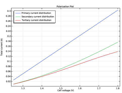
Figure 2 shows the different polarization plots that results from using a parametric solver to solve for all the three cases of current distribution. The total current decreases as potential losses due to kinetics and mass transport are introduced in the model. The following sections cover each case more in detail.
Figure 2: Polarization plots comparing the three cases of current distribution.
PRIMARY CURRENT DISTRIBUTION
Figure 3 shows the potential distribution in the electrolyte and current density distribution at the anode at a cell voltage of 1.45 V. The current density distribution is highest at the corners of the wires and close to zero at the central parts of the wire structure.
Figure 3: Primary current distribution, Ecell=1.45 V. Potential distribution in the electrolyte (top) and current density on the anode (bottom).
SECONDARY CURRENT DISTRIBUTION
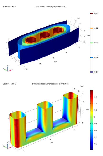
Figure 4 shows the plots for the secondary current distribution. A higher cell voltage is chosen reach a total cell current comparable to Figure 3. Compared to the primary current distribution the secondary current distribution is smoother, this is due to the effect that a high local current density induces local overpotential losses on the electrode surface.
Figure 4: Secondary current distribution, Ecell=1.65 V. Potential distribution in the electrolyte (left) and current density on the anode (right).
TERTIARY CURRENT DSITRIBUTION
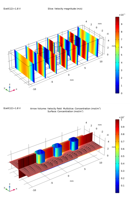
Figure 5 shows the flow velocity magnitude of the flow and the concentration of the reactant at 1.8 V. The convective flow is close to zero between the wires, and this results in a depletion zone with low concentration in these parts in the cell.
Figure 5: Flow field (top: slice plot, right: arrows) and concentration profile (bottom: slices and anode surface) at 1.8 V.
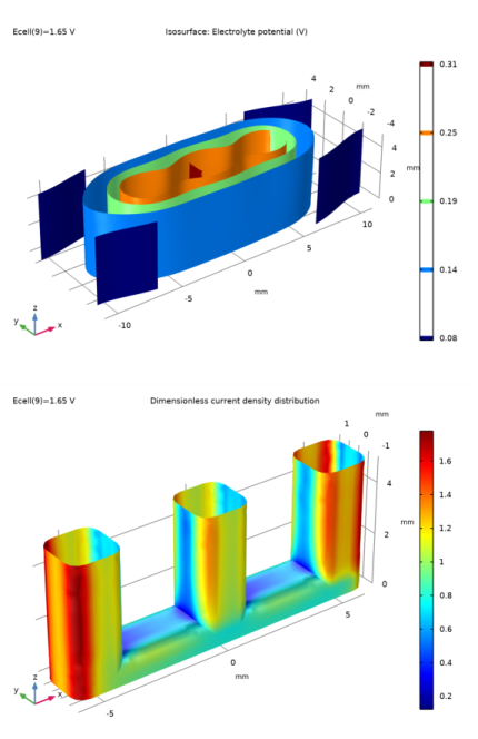
Figure 6 shows the resulting potential and current density distribution. The low concentration between the wires now impacts severely on the smoothness of the current distribution.
Figure 6: Tertiary current distribution, Ecell=1.65 V. Potential distribution in the electrolyte (top) and current density on the anode (bottom).
Notes About the COMSOL Implementation
You set up the model using the following physics interfaces:
Primary Current Distribution for modeling the electrolyte potential, governed by Ohm’s Law (Equation 3). The secondary and tertiary current distributions are modeled by changing the current distribution type of the interface to Secondary.
References
1. J.S. Newman, Electrochemical Systems, 2nd ed., Prentice Hall, NJ, 1990.
2. J. O’M. Bockris and A.K.N. Reddy, Modern Electrochemistry, Plenum Press, NY, 1970.
Application Library path: Electrochemistry_Module/Electrochemical_Engineering/wire_electrode
Modeling Instructions
From the File menu, choose New.
New
In the New window, click  Model Wizard.
Model Wizard
1
In the Model Wizard window, click  3D.
2
In the Select Physics tree, select Electrochemistry>Primary and Secondary Current Distribution>Primary Current Distribution (cd).
3
Click Add.
4
Click  Study.
5
In the Select Study tree, select General Studies>Stationary.
6
Geometry 1
The model geometry is available as a parameterized geometry sequence in a separate MPH-file. If you want to build it from scratch, follow the instructions in the section Appendix — Geometry Modeling Instructions. Otherwise load it from file with the following steps.
1
In the Geometry toolbar, click  Insert Sequence.
2
3
In the Geometry toolbar, click  Build All.
Global Definitions
Now start defining the physics for the primary current distribution simulation. Begin with the model parameters.
Parameters 1
1
In the Model Builder window, under Global Definitions click Parameters 1.
2
In the Settings window for Parameters, locate the Parameters section.
3
Materials
Add water from the material library. Modify the material by adding the conductivity value.
Add Material
1
In the Home toolbar, click  Add Material to open the Add Material window.
2
Go to the Add Material window.
3
In the tree, select Built-in>Water, liquid.
4
Click Add to Component in the window toolbar.
5
In the Home toolbar, click  Add Material to close the Add Material window.
Materials
Electrolyte
1
In the Settings window for Material, locate the Material Contents section.
2
3
Right-click Component 1 (comp1)>Materials>Water, liquid (mat1) and choose Rename.
4
In the Rename Material dialog box, type Electrolyte in the New label text field.
5
Primary Current Distribution (cd)
Electrolyte 1
Now start setting up the physics. Only the equilibrium potentials and the electrode potential boundary values need to be set for the primary current distribution.
Electrode Surface 1
1
In the Model Builder window, right-click Primary Current Distribution (cd) and choose Electrode Surface.
2
Create selections for these anodes. The selection will be used later when setting up more physics, meshing, and postprocessing.
3
In the Settings window for Electrode Surface, locate the Boundary Selection section.
4
Click  Create Selection.
5
In the Create Selection dialog box, type Cathodes in the Selection name text field.
6
Electrode Reaction 1
1
In the Model Builder window, expand the Electrode Surface 1 node, then click Electrode Reaction 1.
2
In the Settings window for Electrode Reaction, locate the Equilibrium Potential section.
3
In the Eeq text field, type Eeq_c.
Electrode Surface 2
1
In the Physics toolbar, click  Boundaries and choose Electrode Surface.
2
This selection is easiest to achieve by selecting all boundaries (the ’All boundaries’ check box), followed by deselecting all exterior surfaces.
3
In the Settings window for Electrode Surface, locate the Boundary Selection section.
4
Click  Create Selection.
5
In the Create Selection dialog box, type Anode in the Selection name text field.
6
7
In the Settings window for Electrode Surface, locate the Electrode Phase Potential Condition section.
8
In the φs,ext text field, type Ecell.
Electrode Reaction 1
1
In the Model Builder window, expand the Electrode Surface 2 node, then click Electrode Reaction 1.
2
In the Settings window for Electrode Reaction, locate the Equilibrium Potential section.
3
In the Eeq text field, type Eeq_a.
Initial Values 1
Also, provide initial values for the electrolyte potential.
1
In the Model Builder window, click Initial Values 1.
2
In the Settings window for Initial Values, locate the Initial Values section.
3
In the phil text field, type (Ecell-Eeq_a-Eeq_c)/2.
Mesh 1
The following steps create a mesh with boundary layers adjacent to the anode and cathode surfaces. This is a convenient way of increasing the number of mesh elements close to a surface of special interest.
Boundary Layers 1
In the Mesh toolbar, click  Boundary Layers.
Boundary Layer Properties
1
In the Model Builder window, click Boundary Layer Properties.
2
In the Settings window for Boundary Layer Properties, locate the Geometric Entity Selection section.
3
From the Selection list, choose Anode.
4
Locate the Boundary Layer Properties section. In the Number of boundary layers text field, type 6.
5
In the Boundary layer stretching factor text field, type 1.3.
6
From the Thickness of first layer list, choose Manual.
7
In the Thickness text field, type 2e-5[m].
Boundary Layer Properties 1
1
In the Mesh toolbar, click  More Attributes and choose Boundary Layer Properties.
2
In the Settings window for Boundary Layer Properties, locate the Boundary Selection section.
3
From the Selection list, choose Cathodes.
4
Locate the Boundary Layer Properties section. In the Number of boundary layers text field, type 2.
5
In the Boundary layer stretching factor text field, type 1.3.
6
In the Thickness adjustment factor text field, type 5.
Size
1
In the Model Builder window, click Size.
2
In the Settings window for Size, locate the Element Size section.
3
From the Calibrate for list, choose Fluid dynamics.
Definitions
Before solving, create some component couplings to be used when analyzing the results.
Integration 1 (intop1)
1
In the Definitions toolbar, click  Nonlocal Couplings and choose Integration.
2
In the Settings window for Integration, type anode_int in the Operator name text field.
3
Locate the Source Selection section. From the Geometric entity level list, choose Boundary.
4
From the Selection list, choose Anode.
Average 1 (aveop1)
1
In the Definitions toolbar, click  Nonlocal Couplings and choose Average.
2
In the Settings window for Average, type anode_avg in the Operator name text field.
3
Locate the Source Selection section. From the Geometric entity level list, choose Boundary.
4
From the Selection list, choose Anode.
Study 1
The model is now ready for solving. Add an auxiliary continuation sweep to solve for a range of cell potentials.
Step 1: Stationary
1
In the Model Builder window, under Study 1 click Step 1: Stationary.
2
In the Settings window for Stationary, click to expand the Study Extensions section.
3
Select the Auxiliary sweep check box.
4
5
6
In the Model Builder window, click Study 1.
7
In the Settings window for Study, locate the Study Settings section.
8
Clear the Generate default plots check box.
9
In the Home toolbar, click  Compute.
You have now solved the primary current distribution model.
Solution 1 (sol1)
To store this particular primary current distribution solution from the latest computation, copy and store the solution in order to compare with these results later when you modify the model.
1
In the Model Builder window, expand the Study 1>Solver Configurations node.
2
Right-click Solution 1 (sol1) and choose Solution>Copy.
Primary current distribution
1
In the Model Builder window, under Study 1>Solver Configurations click Solution 1 - Copy 1 (sol2).
2
In the Settings window for Solution, type Primary current distribution in the Label text field.
Results
Polarization Plot
Now create a polarization plot for the primary current distribution model.
1
In the Home toolbar, click  Add Plot Group and choose 1D Plot Group.
2
In the Settings window for 1D Plot Group, type Polarization Plot in the Label text field.
3
Locate the Data section. From the Dataset list, choose None.
4
Click to expand the Title section. From the Title type list, choose Label.
5
Locate the Plot Settings section. Select the x-axis label check box.
6
7
Select the y-axis label check box.
8
9
Locate the Legend section. From the Position list, choose Upper left.
Global 1
1
Right-click Polarization Plot and choose Global.
2
In the Settings window for Global, locate the Data section.
3
From the Dataset list, choose Study 1/Primary current distribution (sol2).
4
Locate the y-Axis Data section. In the table, enter the following settings:
5
Click to expand the Legends section. From the Legends list, choose Manual.
6
7
In the Polarization Plot toolbar, click  Plot.
Electrolyte Potential
The following creates an isosurface of the potential in the electrolyte.
1
In the Home toolbar, click  Add Plot Group and choose 3D Plot Group.
2
In the Settings window for 3D Plot Group, type Electrolyte Potential in the Label text field.
3
Locate the Data section. From the Dataset list, choose Study 1/Primary current distribution (sol2).
4
From the Parameter value (Ecell (V)) list, choose 1.45.
5
Locate the Plot Settings section. Clear the Plot dataset edges check box.
Isosurface 1
1
Right-click Electrolyte Potential and choose Isosurface.
2
In the Electrolyte Potential toolbar, click  Plot.
3
Click the  Zoom Extents button in the Graphics toolbar.
Dimensionless current density distribution
The following creates a normalized plot of the normal electrolyte current density on the anode surface.
1
In the Home toolbar, click  Add Plot Group and choose 3D Plot Group.
2
In the Settings window for 3D Plot Group, type Dimensionless current density distribution in the Label text field.
3
Locate the Data section. From the Dataset list, choose Study 1/Primary current distribution (sol2).
4
From the Parameter value (Ecell (V)) list, choose 1.45.
5
Click to expand the Selection section. From the Geometric entity level list, choose Boundary.
6
From the Selection list, choose Anode.
7
Click to expand the Title section. From the Title type list, choose Label.
8
Locate the Plot Settings section. Clear the Plot dataset edges check box.
Surface 1
1
Right-click Dimensionless current density distribution and choose Surface.
Plot the normal current density divided by the average normal current density.
2
In the Settings window for Surface, locate the Expression section.
3
In the Expression text field, type (comp1.cd.nIl)/anode_avg(comp1.cd.nIl).
4
In the Dimensionless current density distribution toolbar, click  Plot.
5
Click the  Zoom Extents button in the Graphics toolbar.
Primary Current Distribution (cd)
Now modify the model to simulate the secondary current distribution.
1
In the Model Builder window, under Component 1 (comp1) click Primary Current Distribution (cd).
2
In the Settings window for Primary Current Distribution, locate the Current Distribution Type section.
3
From the Current distribution type list, choose Secondary.
Global Definitions
Parameters 1
Add the needed parameters for the secondary model.
1
In the Model Builder window, under Global Definitions click Parameters 1.
2
In the Settings window for Parameters, locate the Parameters section.
3
Secondary Current Distribution (cd)
Electrode Reaction 1
Now set up the new boundary conditions for the secondary current distribution by adding the needed kinetic parameters for Electrode Reaction 1 (er1) in Electrode Surface 1 (es1) node.
1
In the Model Builder window, under Component 1 (comp1)>Secondary Current Distribution (cd)>Electrode Surface 1 click Electrode Reaction 1.
2
In the Settings window for Electrode Reaction, locate the Electrode Kinetics section.
3
From the Kinetics expression type list, choose Butler-Volmer.
4
In the i0 text field, type i0_c.
5
In the αa text field, type be_c.
6
In the αc text field, type 1-be_c.
Similarly, define the kinetic parameters at the anode for Electrode Reaction 1 (er1) in Electrode Surface 2 (es2) node.
Electrode Reaction 1
1
In the Model Builder window, click Electrode Reaction 1.
2
In the Settings window for Electrode Reaction, locate the Electrode Kinetics section.
3
From the Kinetics expression type list, choose Butler-Volmer.
4
In the i0 text field, type i0_a.
5
In the αa text field, type be_a.
6
In the αc text field, type 1-be_a.
Global Definitions
Default Model Inputs
Set up the temperature value used in the entire model.
1
In the Model Builder window, under Global Definitions click Default Model Inputs.
2
In the Settings window for Default Model Inputs, locate the Browse Model Inputs section.
3
In the tree, select General>Temperature (K) - minput.T.
4
Find the Expression for remaining selection subsection. In the Temperature text field, type T.
Study 1
In the Home toolbar, click  Compute.
Results
Electrolyte Potential
You have now solved the secondary current distribution problem.
Study 1
Secondary current distribution
1
In the Model Builder window, under Study 1>Solver Configurations click Solution 1 (sol1).
2
In the Settings window for Solution, type Secondary current distribution in the Label text field.
Results
Proceed to look at the results by adding the secondary current distribution polarization plot.
Global 2
1
In the Model Builder window, under Results>Polarization Plot right-click Global 1 and choose Duplicate.
2
In the Settings window for Global, locate the Data section.
3
From the Dataset list, choose Study 1/Secondary current distribution (sol1).
4
Locate the Legends section. In the table, enter the following settings:
Polarization Plot
1
In the Model Builder window, click Polarization Plot.
2
In the Polarization Plot toolbar, click  Plot.
Electrolyte Potential
Note the 3D plots are now showing the results of the latest computation. (By choosing different datasets you may compare the primary and secondary current distribution results.)
1
In the Model Builder window, click Electrolyte Potential.
2
In the Settings window for 3D Plot Group, locate the Data section.
3
From the Parameter value (Ecell (V)) list, choose 1.65.
4
In the Electrolyte Potential toolbar, click  Plot.
5
Click the  Zoom Extents button in the Graphics toolbar.
Dimensionless current density distribution
1
In the Model Builder window, click Dimensionless current density distribution.
2
In the Settings window for 3D Plot Group, locate the Data section.
3
From the Parameter value (Ecell (V)) list, choose 1.65.
4
In the Dimensionless current density distribution toolbar, click  Plot.
5
Click the  Zoom Extents button in the Graphics toolbar.
Global Definitions
Now modify the problem to model a tertiary current distribution problem by adding mass transport. Start by adding the parameters.
Parameters 1
1
In the Model Builder window, under Global Definitions click Parameters 1.
2
In the Settings window for Parameters, locate the Parameters section.
3
Add Physics
1
In the Home toolbar, click  Add Physics to open the Add Physics window.
2
Go to the Add Physics window.
3
In the tree, select Chemical Species Transport>Transport of Diluted Species (tds).
4
Click Add to Component 1 in the window toolbar.
5
In the tree, select Fluid Flow>Single-Phase Flow>Laminar Flow (spf).
6
Click Add to Component 1 in the window toolbar.
7
In the Home toolbar, click  Add Physics to close the Add Physics window.
Transport of Diluted Species (tds)
1
In the Model Builder window, under Component 1 (comp1) click Transport of Diluted Species (tds).
2
In the Settings window for Transport of Diluted Species, locate the Transport Mechanisms section.
3
Select the Migration in electric field check box.
Transport Properties 1
The velocity field will be coupled to Laminar Flow later using the Reacting Flow multiphysics feature.
1
In the Model Builder window, under Component 1 (comp1)>Transport of Diluted Species (tds) click Transport Properties 1.
2
In the Settings window for Transport Properties, locate the Diffusion section.
3
In the Dc text field, type D.
The migration potential will be coupled to Secondary Current Distribution later using the Potential Coupling multiphysics feature.
4
Locate the Migration in Electric Field section. In the zc text field, type -1.
Inflow 1
1
In the Physics toolbar, click  Boundaries and choose Inflow.
2
3
In the Settings window for Inflow, locate the Boundary Selection section.
4
Click  Create Selection.
5
In the Create Selection dialog box, type Inlet in the Selection name text field.
6
7
In the Settings window for Inflow, locate the Concentration section.
8
In the c0,c text field, type c_in.
Outflow 1
1
In the Physics toolbar, click  Boundaries and choose Outflow.
2
3
In the Settings window for Outflow, locate the Boundary Selection section.
4
Click  Create Selection.
5
In the Create Selection dialog box, type Outlet in the Selection name text field.
6
Initial Values 1
1
In the Model Builder window, click Initial Values 1.
2
In the Settings window for Initial Values, locate the Initial Values section.
3
In the c text field, type c_in.
Electrode Surface Coupling 1
Couple the flux on the anode surface to the electrode reaction currents by using a Electrode-Electrolyte Interface Coupling feature.
1
In the Physics toolbar, click  Boundaries and choose Electrode Surface Coupling.
2
In the Settings window for Electrode Surface Coupling, locate the Boundary Selection section.
3
From the Selection list, choose Anode.
Reaction Coefficients 1
1
In the Model Builder window, expand the Electrode Surface Coupling 1 node, then click Reaction Coefficients 1.
2
In the Settings window for Reaction Coefficients, locate the Model Inputs section.
3
From the iloc list, choose Local current density, Electrode Reaction 1 (cd/es2/er1).
4
Locate the Stoichiometric Coefficients section. In the νc text field, type 1.
Secondary Current Distribution (cd)
Also modify the current density expression to be concentration dependent.
Electrode Reaction 1
1
In the Model Builder window, under Component 1 (comp1)>Secondary Current Distribution (cd)>Electrode Surface 2 click Electrode Reaction 1.
2
In the Settings window for Electrode Reaction, locate the Equilibrium Potential section.
3
From the Eeq list, choose Nernst equation.
4
In the Eeq,ref(T) text field, type Eeq_a.
5
In the CR text field, type c/c_in.
6
Locate the Electrode Kinetics section. From the Exchange current density type list, choose From Nernst Equation.
7
In the i0,ref(T) text field, type i0_a.
Laminar Flow (spf)
In the Model Builder window, under Component 1 (comp1) click Laminar Flow (spf).
Inlet 1
1
In the Physics toolbar, click  Boundaries and choose Inlet.
2
In the Settings window for Inlet, locate the Boundary Selection section.
3
From the Selection list, choose Inlet.
4
Locate the Boundary Condition section. From the list, choose Fully developed flow.
5
Locate the Fully Developed Flow section. In the Uav text field, type u_in.
Outlet 1
1
In the Physics toolbar, click  Boundaries and choose Outlet.
2
In the Settings window for Outlet, locate the Boundary Selection section.
3
From the Selection list, choose Outlet.
4
Locate the Pressure Conditions section. Select the Normal flow check box.
Wall 2
1
In the Physics toolbar, click  Boundaries and choose Wall.
2
3
In the Settings window for Wall, locate the Boundary Condition section.
4
From the Wall condition list, choose Slip.
Multiphysics
Finally, set up the Reacting Flow and Potential Coupling multiphysics features.
Reacting Flow, Diluted Species 1 (rfd1)
In the Physics toolbar, click  Multiphysics Couplings and choose Domain>Reacting Flow, Diluted Species.
Potential Coupling 1 (pc1)
1
In the Physics toolbar, click  Multiphysics Couplings and choose Domain>Potential Coupling.
2
Root
Next, set up the solver for the tertiary current distribution problem. Do this by adding a new study wherein you first solve for the flow problem, which does not depend on the other variables, and then the species transport and electric currents.
Add Study
1
In the Home toolbar, click  Add Study to open the Add Study window.
2
Go to the Add Study window.
3
Find the Studies subsection. In the Select Study tree, select General Studies>Stationary.
4
Click Add Study in the window toolbar.
5
In the Home toolbar, click  Add Study to close the Add Study window.
Study 2
Step 1: Stationary
1
In the Settings window for Stationary, locate the Physics and Variables Selection section.
2
In the table, clear the Solve for check boxes for Secondary Current Distribution (cd) and Transport of Diluted Species (tds).
Stationary 2
1
In the Study toolbar, click  Study Steps and choose Stationary>Stationary.
2
In the Settings window for Stationary, locate the Physics and Variables Selection section.
3
In the table, clear the Solve for check box for Laminar Flow (spf).
Set up an auxiliary continuation sweep for the Ecell parameter.
4
Click to expand the Study Extensions section. Select the Auxiliary sweep check box.
5
6
Solution 3 (sol3)
Change to a fully coupled direct solver to decrease solver time.
1
In the Study toolbar, click  Show Default Solver.
2
In the Model Builder window, expand the Solution 3 (sol3) node.
3
In the Model Builder window, expand the Study 2>Solver Configurations>Solution 3 (sol3)>Stationary Solver 2 node.
4
Right-click Stationary Solver 2 and choose Fully Coupled.
5
In the Settings window for Fully Coupled, locate the General section.
6
From the Linear solver list, choose Direct (cd).
7
In the Model Builder window, click Study 2.
8
In the Settings window for Study, locate the Study Settings section.
9
Clear the Generate default plots check box.
10
In the Study toolbar, click  Compute.
You have now solved the tertiary current distribution.
11
In the Label text field, type Tertiary current distribution.
Results
Add the tertiary current distribution to the polarization plot.
Global 3
1
In the Model Builder window, under Results>Polarization Plot right-click Global 2 and choose Duplicate.
2
In the Settings window for Global, locate the Data section.
3
From the Dataset list, choose Tertiary current distribution/Solution 3 (sol3).
4
Locate the Legends section. In the table, enter the following settings:
5
In the Polarization Plot toolbar, click  Plot.
Velocity
1
In the Home toolbar, click  Add Plot Group and choose 3D Plot Group.
2
In the Settings window for 3D Plot Group, type Velocity in the Label text field.
3
Locate the Data section. From the Dataset list, choose Tertiary current distribution/Solution 3 (sol3).
Slice 1
1
Right-click Velocity and choose Slice.
2
In the Settings window for Slice, click Replace Expression in the upper-right corner of the Expression section. From the menu, choose Component 1 (comp1)>Laminar Flow>Velocity and pressure>spf.U - Velocity magnitude - m/s.
3
Locate the Plane Data section. In the Planes text field, type 7.
4
In the Velocity toolbar, click  Plot.
5
Click the  Zoom Extents button in the Graphics toolbar.
Concentration
Finish the postprocessing by creating an arrow, slice, and surface plot that visualizes the concentration and flow in the cell.
1
In the Home toolbar, click  Add Plot Group and choose 3D Plot Group.
2
In the Settings window for 3D Plot Group, type Concentration in the Label text field.
3
Locate the Data section. From the Dataset list, choose Tertiary current distribution/Solution 3 (sol3).
4
Locate the Plot Settings section. Clear the Plot dataset edges check box.
Arrow Volume 1
1
Right-click Concentration and choose Arrow Volume.
2
In the Settings window for Arrow Volume, click Replace Expression in the upper-right corner of the Expression section. From the menu, choose Component 1 (comp1)>Laminar Flow>Velocity and pressure>u,v,w - Velocity field.
3
Locate the Arrow Positioning section. Find the x grid points subsection. In the Points text field, type 15.
4
Find the y grid points subsection. In the Points text field, type 15.
5
Find the z grid points subsection. In the Points text field, type 1.
6
Locate the Coloring and Style section. From the Color list, choose Black.
Arrow Volume 2
1
Right-click Arrow Volume 1 and choose Duplicate.
2
In the Settings window for Arrow Volume, click to expand the Title section.
3
From the Title type list, choose None.
4
Locate the Arrow Positioning section. Find the y grid points subsection. In the Points text field, type 1.
5
Find the z grid points subsection. In the Points text field, type 15.
6
Click to expand the Inherit Style section. From the Plot list, choose Arrow Volume 1.
7
In the Concentration toolbar, click  Plot.
Concentration
In the Model Builder window, click Concentration.
Multislice 1
1
In the Concentration toolbar, click  More Plots and choose Multislice.
2
In the Settings window for Multislice, click Replace Expression in the upper-right corner of the Expression section. From the menu, choose Component 1 (comp1)>Transport of Diluted Species>Species c>c - Concentration - mol/m³.
3
Locate the Multiplane Data section. Find the x-planes subsection. In the Planes text field, type 0.
Surface 1
1
Right-click Concentration and choose Surface.
2
In the Settings window for Surface, click Replace Expression in the upper-right corner of the Expression section. From the menu, choose Component 1 (comp1)>Transport of Diluted Species>Species c>c - Concentration - mol/m³.
3
Click to expand the Inherit Style section. From the Plot list, choose Multislice 1.
Selection 1
1
Right-click Surface 1 and choose Selection.
2
In the Settings window for Selection, locate the Selection section.
3
From the Selection list, choose Anode.
4
In the Concentration toolbar, click  Plot.
Electrolyte Potential
1
In the Model Builder window, click Electrolyte Potential.
2
In the Settings window for 3D Plot Group, locate the Data section.
3
From the Dataset list, choose Tertiary current distribution/Solution 3 (sol3).
4
In the Electrolyte Potential toolbar, click  Plot.
Dimensionless current density distribution
1
In the Model Builder window, click Dimensionless current density distribution.
2
In the Settings window for 3D Plot Group, locate the Data section.
3
From the Dataset list, choose Tertiary current distribution/Solution 3 (sol3).
4
In the Dimensionless current density distribution toolbar, click  Plot.
5
Click the  Zoom Extents button in the Graphics toolbar.
Appendix — Geometry Modeling Instructions
From the File menu, choose New.
New
In the New window, click  Blank Model.
Add Component
In the Home toolbar, click  Add Component and choose 3D.
Geometry 1
1
In the Settings window for Geometry, locate the Units section.
2
From the Length unit list, choose mm.
Block 1 (blk1)
In the Geometry toolbar, click  Block.
Definitions
View 1
1
In the Model Builder window, expand the Component 1 (comp1)>Definitions node, then click View 1.
2
In the Settings window for View, locate the View section.
3
Select the Wireframe rendering check box.
Geometry 1
Block 1 (blk1)
1
In the Model Builder window, under Component 1 (comp1)>Geometry 1 click Block 1 (blk1).
2
In the Settings window for Block, locate the Size and Shape section.
3
In the Width text field, type 22.
4
In the Depth text field, type 8.
5
In the Height text field, type 5.
6
Locate the Position section. In the x text field, type -11.
7
In the y text field, type -4.
Cumulative Selections
In the Geometry toolbar, click  Selections and choose Cumulative Selections.
Union
1
Right-click Cumulative Selections and choose Cumulative Selection.
2
In the Settings window for Selection, type Union in the Label text field.
Work Plane 1 (wp1)
1
In the Geometry toolbar, click  Work Plane.
2
In the Settings window for Work Plane, locate the Plane Definition section.
3
In the z-coordinate text field, type -1.
Work Plane 1 (wp1)>Plane Geometry
In the Model Builder window, click Plane Geometry.
Work Plane 1 (wp1)>Square 1 (sq1)
1
In the Work Plane toolbar, click  Square.
2
In the Settings window for Square, locate the Size section.
3
In the Side length text field, type 2.
4
Locate the Position section. In the xw text field, type -6.
5
In the yw text field, type -1.
6
Locate the Selections of Resulting Entities section. Select the Resulting objects selection check box.
Work Plane 1 (wp1)>Fillet 1 (fil1)
1
In the Work Plane toolbar, click  Fillet.
2
On the object sq1, select Points 1–4 only.
3
In the Settings window for Fillet, locate the Radius section.
4
In the Radius text field, type 0.5.
5
Locate the Selections of Resulting Entities section. Select the Resulting objects selection check box.
Work Plane 1 (wp1)>Array 1 (arr1)
1
In the Work Plane toolbar, click  Transforms and choose Array.
2
3
In the Settings window for Array, locate the Size section.
4
In the xw size text field, type 3.
5
Locate the Displacement section. In the xw text field, type 5.
Extrude 1 (ext1)
1
In the Model Builder window, expand the Component 1 (comp1)>Geometry 1>Work Plane 1 (wp1)>View 2 node.
2
Right-click Geometry 1 and choose Extrude.
3
In the Settings window for Extrude, locate the Distances section.
4
5
Locate the Selections of Resulting Entities section. Find the Cumulative selection subsection. From the Contribute to list, choose Union.
Work Plane 2 (wp2)
1
In the Geometry toolbar, click  Work Plane.
2
In the Settings window for Work Plane, locate the Plane Definition section.
3
From the Plane list, choose yz-plane.
4
In the x-coordinate text field, type 11.
Work Plane 2 (wp2)>Plane Geometry
In the Model Builder window, click Plane Geometry.
Work Plane 2 (wp2)>Square 1 (sq1)
1
In the Work Plane toolbar, click  Square.
2
In the Settings window for Square, locate the Size section.
3
In the Side length text field, type 2.
4
Locate the Position section. From the Base list, choose Center.
5
Locate the Selections of Resulting Entities section. Select the Resulting objects selection check box.
Work Plane 2 (wp2)>Fillet 1 (fil1)
1
In the Work Plane toolbar, click  Fillet.
2
On the object sq1, select Points 1–4 only.
3
In the Settings window for Fillet, locate the Radius section.
4
In the Radius text field, type 0.5.
Extrude 2 (ext2)
1
In the Model Builder window, expand the Component 1 (comp1)>Geometry 1>Work Plane 2 (wp2)>View 3 node.
2
Right-click Geometry 1 and choose Extrude.
3
In the Settings window for Extrude, locate the Distances section.
4
5
Select the Reverse direction check box.
6
Locate the Selections of Resulting Entities section. Find the Cumulative selection subsection. From the Contribute to list, choose Union.
Union 1 (uni1)
1
In the Geometry toolbar, click  Booleans and Partitions and choose Union.
2
In the Settings window for Union, locate the Union section.
3
From the Input objects list, choose Union.
Delete Entities 1 (del1)
1
Right-click Geometry 1 and choose Delete Entities.
2
In the Settings window for Delete Entities, locate the Entities or Objects to Delete section.
3
From the Geometric entity level list, choose Domain.
4
Click the  Zoom Extents button in the Graphics toolbar.
5
On the object uni1, select Domains 1 and 16 only.
6
Locate the Selections of Resulting Entities section. Select the Resulting objects selection check box.
Union 2 (uni2)
1
In the Geometry toolbar, click  Booleans and Partitions and choose Union.
2
In the Settings window for Union, locate the Union section.
3
From the Input objects list, choose Delete Entities 1.
Difference 1 (dif1)
1
In the Geometry toolbar, click  Booleans and Partitions and choose Difference.
2
Union 2 (uni2)
1
In the Model Builder window, click Union 2 (uni2).
2
In the Settings window for Union, locate the Selections of Resulting Entities section.
3
Select the Resulting objects selection check box.
Difference 1 (dif1)
1
In the Model Builder window, click Difference 1 (dif1).
2
In the Settings window for Difference, locate the Difference section.
3
From the Objects to subtract list, choose Union 2.
Box Selection 1 (boxsel1)
1
In the Geometry toolbar, click  Selections and choose Box Selection.
2
In the Settings window for Box Selection, locate the Geometric Entity Level section.
3
From the Level list, choose Boundary.
4
Locate the Box Limits section. In the x minimum text field, type -60.
5
In the x maximum text field, type 60.
6
In the y minimum text field, type -2.
7
In the y maximum text field, type 2.
Cathodes
1
In the Geometry toolbar, click  Selections and choose Explicit Selection.
2
In the Settings window for Explicit Selection, type Cathodes in the Label text field.
3
Locate the Entities to Select section. From the Geometric entity level list, choose Boundary.
Anode
1
In the Model Builder window, under Component 1 (comp1)>Geometry 1 click Box Selection 1 (boxsel1).
2
In the Settings window for Box Selection, type Anode in the Label text field.
3
Locate the Output Entities section. From the Include entity if list, choose Entity inside box.
Cathodes (sel1)
1
In the Model Builder window, click Cathodes (sel1).
2
In the Settings window for Explicit Selection, locate the Entities to Select section.
3
Find the Entities to select subsection. Select the  Activate Selection toggle button.
4
On the object dif1, select Boundaries 2 and 5 only.
Anode (boxsel1), Cathodes (sel1)
1
In the Model Builder window, under Component 1 (comp1)>Geometry 1, Ctrl-click to select Anode (boxsel1) and Cathodes (sel1).
2
Inlet
1
In the Geometry toolbar, click  Selections and choose Explicit Selection.
2
In the Settings window for Explicit Selection, type Inlet in the Label text field.
3
Click the  Zoom Extents button in the Graphics toolbar.
4
Locate the Entities to Select section. From the Geometric entity level list, choose Boundary.
5
On the object fin, select Boundary 1 only.
Outlet
1
In the Geometry toolbar, click  Selections and choose Explicit Selection.
2
In the Settings window for Explicit Selection, type Outlet in the Label text field.
3
Locate the Entities to Select section. From the Geometric entity level list, choose Boundary.
4
On the object fin, select Boundary 52 only.
5
In the Geometry toolbar, click  Build All.