|
|
|

|
1
|
|
2
|
In the Select Physics tree, select Electrochemistry>Primary and Secondary Current Distribution>Secondary Current Distribution (cd).
|
|
3
|
Click Add.
|
|
4
|
Click
|
|
5
|
|
6
|
Click
|
|
1
|
|
2
|
|
3
|
Click Browse.
|
|
4
|
Browse to the model’s Application Libraries folder and double-click the file ship_hull_geometry.mphbin.
|
|
5
|
Click Import.
|
|
1
|
|
2
|
On the object fin, select Boundaries 9–12 and 15 only.
|
|
3
|
|
4
|
|
5
|
|
1
|
|
2
|
|
3
|
|
4
|
Browse to the model’s Application Libraries folder and double-click the file ship_hull_parameters.txt.
|
|
1
|
|
2
|
|
3
|
|
4
|
|
5
|
|
6
|
Click OK.
|
|
7
|
|
8
|
|
9
|
Click OK.
|
|
1
|
|
2
|
|
3
|
|
4
|
|
5
|
|
6
|
Click OK.
|
|
7
|
|
8
|
|
9
|
Click OK.
|
|
1
|
|
2
|
|
3
|
|
4
|
|
5
|
|
6
|
Click OK.
|
|
7
|
|
8
|
|
9
|
Click OK.
|
|
1
|
|
2
|
|
3
|
|
4
|
|
5
|
|
6
|
Click OK.
|
|
7
|
|
8
|
|
9
|
Click OK.
|
|
1
|
|
2
|
|
3
|
|
4
|
|
5
|
|
6
|
Click OK.
|
|
7
|
|
8
|
|
9
|
Click OK.
|
|
1
|
|
2
|
|
3
|
|
4
|
|
5
|
|
6
|
Click OK.
|
|
7
|
|
8
|
|
9
|
Click OK.
|
|
1
|
|
2
|
|
3
|
|
4
|
|
5
|
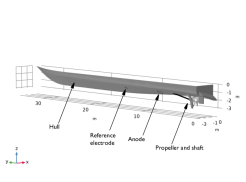
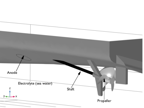
In the Add dialog box, in the Selections to add list, choose Propeller base, Propeller blades, Shaft, Anode, Reference electrode, and Hull surface.
|
|
6
|
Click OK.
|
|
7
|
|
8
|
|
9
|
Click OK.
|
|
1
|
|
2
|
|
3
|
|
4
|
|
5
|
In the Add dialog box, in the Selections to add list, choose Propeller base, Propeller blades, and Shaft.
|
|
6
|
Click OK.
|
|
7
|
|
8
|
|
9
|
Click OK.
|
|
1
|
|
2
|
|
3
|
|
4
|
|
5
|
|
6
|
Click OK.
|
|
7
|
|
8
|
|
9
|
Click OK.
|
|
1
|
|
2
|
|
3
|
|
4
|
|
1
|
|
2
|
|
3
|
|
4
|
|
1
|
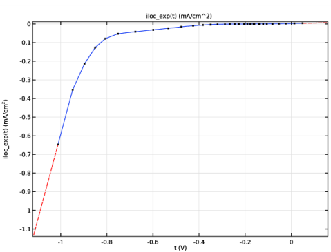
In the Model Builder window, expand the Component 1 (comp1)>Materials>Alloy 625 in seawater at 30 C (mat1)>Local current density (lcd) node, then click Interpolation 1 (iloc_exp).
|
|
2
|
|
1
|
|
2
|
|
3
|
|
1
|
|
2
|
|
3
|
|
4
|
|
1
|
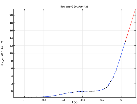
In the Model Builder window, expand the Component 1 (comp1)>Materials>NAB in seawater at 30 C (mat2)>Local current density (lcd) node, then click Interpolation 1 (iloc_exp).
|
|
2
|
|
1
|
|
2
|
In the Settings window for Secondary Current Distribution, click to expand the Physics vs. Materials Reference Electrode Potential section.
|
|
3
|
|
1
|
In the Model Builder window, under Component 1 (comp1)>Secondary Current Distribution (cd) click Electrolyte 1.
|
|
2
|
|
3
|
|
1
|
|
1
|
|
2
|
|
3
|
|
1
|
|
2
|
|
3
|
|
4
|
Locate the Electrode Phase Potential Condition section. From the Electrode phase potential condition list, choose Electrode potential.
|
|
5
|
|
6
|
|
1
|
|
2
|
|
3
|
|
4
|
|
5
|
|
1
|
In the Model Builder window, under Component 1 (comp1) right-click Definitions and choose Variables.
|
|
2
|
|
4
|
Locate the Geometric Entity Selection section. From the Geometric entity level list, choose Boundary.
|
|
5
|
|
6
|
Locate the Variables section. In the table, enter the following settings:
|
|
1
|
|
3
|
|
4
|
|
5
|
|
6
|
Select the xy-plane check box.
|
|
1
|
|
2
|
|
3
|
|
1
|
|
2
|
|
3
|
|
1
|
|
2
|
|
3
|
|
4
|
Click the Custom button.
|
|
5
|
|
7
|
|
1
|
|
2
|
|
3
|
|
4
|
|
5
|
|
1
|
|
2
|
|
3
|
|
4
|
|
5
|
|
6
|
|
1
|
|
2
|
|
3
|
|
1
|
|
1
|
|
2
|
|
3
|
|
1
|
|
2
|
|
3
|
|
4
|
|
1
|
In the Model Builder window, expand the Electrode Potential vs. Adjacent Reference (cd) node, then click Surface 1.
|
|
2
|
|
3
|
|
1
|
|
2
|
|
3
|
|
4
|
|
1
|
|
2
|
|
3
|
|
4
|
Locate the Electrode Phase Potential Condition section. From the Electrode phase potential condition list, choose Electrode potential.
|
|
5
|
|
6
|
|
1
|
|
2
|
|
3
|
|
4
|
|
5
|
|
1
|
|
2
|
|
3
|
|
4
|
Locate the Electrode Phase Potential Condition section. From the Electrode phase potential condition list, choose Electrode potential.
|
|
5
|
|
6
|
|
1
|
In the Model Builder window, expand the Thin Electrode Surface 1 node, then click Electrode Reaction 1.
|
|
2
|
|
3
|
|
4
|
|
5
|
|
1
|
|
2
|
|
3
|
|
4
|
In the Physics and variables selection tree, select Component 1 (comp1)>Secondary Current Distribution (cd)>Electrode Surface 2.
|
|
5
|
Click
|
|
6
|
In the Physics and variables selection tree, select Component 1 (comp1)>Secondary Current Distribution (cd)>Thin Electrode Surface 1.
|
|
7
|
Click
|
|
1
|
|
2
|
|
3
|
|
4
|
|
5
|
|
1
|
|
2
|
|
3
|
|
1
|
|
2
|
|
3
|
|
4
|
|
1
|
In the Model Builder window, expand the Electrode Potential vs. Adjacent Reference (cd) 1 node, then click Surface 1.
|
|
2
|
|
3
|
|
1
|
|
2
|
|
3
|
|
4
|
|
5
|
|
1
|
|
2
|
|
3
|
|
1
|
|
2
|
|
3
|
|
5
|
|
6
|
|
7
|
|
8
|
|
9
|
|
1
|
|
2
|
|
3
|
|
4
|
Locate the Legends section. In the table, enter the following settings:
|
|
1
|
|
2
|
|
3
|
|
4
|
|
1
|
|
2
|
|
3
|
|
4
|
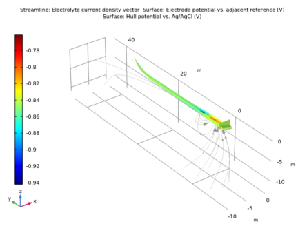
Click Replace Expression in the upper-right corner of the Expressions section. From the menu, choose Component 1 (comp1)>Secondary Current Distribution>cd.nIl - Normal electrolyte current density - A/m².
|
|
5
|
Click
|
|
1
|
|
2
|
|
3
|
|
4
|