PDF

Electrochemical Impedance Spectroscopy
Introduction
Electrochemical impedance spectroscopy is a common technique in electroanalysis. It is used to study the harmonic response of an electrochemical system. A small, sinusoidal variation is applied to the potential at the working electrode, and the resulting current is analyzed in the frequency domain.
The real and imaginary components of the impedance give information about the kinetic and mass transport properties of the cell, as well as its capacitive properties. By measuring impedance at a range of frequencies, the relative influence of the various constituent physics of the system can be interpreted as a function of time scale.
As in electrical analysis, the real component of impedance corresponds to a resistance in-phase with the applied voltage. The imaginary component corresponds to a reactance 90° out-of-phase with the applied voltage; the reactance is caused by capacitive charging in the cell.
Capacitive charging occurs at the double layer adjacent to the working electrode surface. Here, the net charge on the electrode causes accumulation or depletion of charged ions in the neighboring solution; as the potential on the electrode changes, so does its charge, and so the double layer charges and discharges with a characteristic capacitance.
In this example, the AC Impedance, Initial Values study type is used to perform a linearized perturbation study in the frequency domain around the provided initial values to resolve the magnitude and phase of the current response to the sinusoidal voltage. A Parametric Sweep is used to compare the response of the system with different electrode kinetics for the redox couple.
Model Definition
This model contains a single 1D domain. The length of the domain, L (m), is based on the diffusion coefficient, D (m2/s) and lowest frequency, fmin(1/s), in order to be sufficiently large compared to the time scale of diffusion (the diffusion layer).
(1)
DOMAIN EQUATIONS
We assume the presence of a large quantity of supporting electrolyte. This is inert salt that is added in electroanalytical experiments to increase the conductivity of the electrolyte without otherwise interfering with the reaction chemistry. Under these conditions, the resistance of the solution is sufficiently low that the electric field is negligible, and we can assume φl = 0.
The Electroanalysis interface implements chemical transport equations for the reactant and product species of the redox couple subject to this assumption. The domain equation is the diffusion equation (also known as Fick’s 2nd law) to describe the chemical transport of the electroactive species A and B:
BOUNDARY EQUATIONS
Both the oxidized and reduced species are equally concentrated at c = 1 μM in bulk (L).
At the working electrode surface (= 0), the reactant species A oxidizes (loses one electron) to form the product B. By convention, electrochemical reactions are written in the reductive direction:
The stoichiometric coefficient is –1 for B, the “reactant” in the reductive direction, and +1 for A, the “product” in the reductive direction. The number of electrons transferred, n, equals one.
The current density for this reaction is given by the electroanalytical Butler-Volmer equation for an oxidation:
(2)
in which k0 is the heterogeneous rate constant of the reaction, αc is the cathodic transfer coefficient, and η is the overpotential at the working electrode. This overpotential is the difference between the applied potential and the equilibrium potential (formal reduction potential) of the redox couple of species A and B, Eeq:
According to Faraday’s laws of electrolysis, the flux of the reactant and product species are proportional to the current density drawn:
(3)
This is expressed in the Electrode Surface boundary condition.
An additional capacitance is applied at the working electrode. It is set equal to 20 μF/cm2 which is a typical value for a water-metal interface. The real value of this capacitance can be established by impedance spectroscopy of the blank solution containing only the supporting electrolyte, or by an alternative voltammetric method.
AC IMPEDANCE STUDY
The AC Impedance study is used to model a harmonic perturbation applied to a fixed center electrode potential, which in this case is fixed to the equilibrium potential of the redox couple:
where it is implied that only the real part of the complex term contributes.
The magnitude of this perturbation, Δφ, is small with respect to RT/F, so that the Butler-Volmer equation (Equation 2) can be linearized. Therefore, the system responds linearly to the perturbation, and the flux (Equation 3), the concentration profiles, and the current density are all also subject to a sinusoidal perturbation at the same frequency.
The AC Impedance Study makes the approximation that the dependent variables ci can be expressed as the sum of a stationary solution ci,0 due to the center voltage of the applied potential, and a sinusoidal perturbation ci,1 to the concentration resulting from the perturbation on the applied potential:
If ci,1 is complex, it implies that the response of the concentration profile is out-of-phase with the applied waveform.
The AC Impedance Initial Values study contains a Frequency Domain study step that solves for the perturbation around the provided initial values, for a range of applied frequencies from 1 Hz to 1 kHz. In each case the domain equation is the frequency domain form of Fick’s 2nd Law:
solved subject to ci,1 = 0 in bulk and:
at the surface.
A Parametric Sweep is used to investigate different values of the heterogeneous rate constant of the electrode reaction, k0, from a value that is kinetically fast on the time scale of the study (0.1 cm/s) to one that it is slow on the same time scale (0.001 cm/s).
Results and Discussion
A Nyquist plot (Figure 1) is the most common means of plotting the results of an impedance experiment. It is an Argand diagram of the complex value of the impedance as a function of frequency; the real component of impedance (resistance) is plotted on the x-axis, and the imaginary component (reactance) is plotted on the y-axis.
For a fast electrochemical reaction with respect to the frequency of the electrochemical impedance study, the impedance always results from the limitation to the current due to the finite diffusivity of the redox species in the solution. It is known from theory that the real and imaginary impedances are linearly correlated in this “transport-controlled” regime (Figure 1).
For a slow electrochemical reaction with respect to the frequency, the mass transport is unimportant as the rate of electron transfer is limited by the rate of reaction at the surface: this is the “kinetically controlled” regime. This regime is characterized by a semi-circular Nyquist plot.
It is common to observe both regimes in a single plot, since the relevant time scale of the experiment changes with the frequency of the harmonic perturbation. At low frequency, mass transport dominates, but at high frequency (toward the lower-left of the plot), there is a transition to kinetic control. This transition is most marked for the slowest electrochemical reaction studied, where k0 = 0.001 cm/s.
Figure 1: Nyquist plot showing the relation of real to imaginary impedance for a range of frequencies and a range of electrode kinetic heterogeneous rate constants.
In a Bode plot, either the magnitude (Figure 2) or the phase (Figure 3) of the complex impedance is plotted against frequency on the x-axis.
Figure 2: Bode plot showing the magnitude of impedance as a function of frequency for a range of electrode kinetic heterogeneous rate constants.
Figure 3: Bode plot showing the phase of the impedance as a function of frequency for a range of electrode kinetic heterogeneous rate constants.
Depending on whether a reaction proceeds under kinetic or transport control at a certain frequency, the Bode plots have different characteristic appearances. Ref. 1. gives a comprehensive discussion and references to further literature concerning the analysis of electrochemical impedance spectra.
Reference
1. A.J. Bard and L.R. Faulkner, Electrochemical Methods, Fundamentals and Applications, 2nd ed., Wiley, New York, 2001.
Application Library path: Corrosion_Module/General_Electrochemistry/impedance_spectroscopy
Modeling Instructions
From the File menu, choose New.
New
In the New window, click Model Wizard ().
Model Wizard
1
In the Model Wizard window, click 1D ().
2
In the Select Physics tree, select Electrochemistry>Electroanalysis (tcd).
3
Click Add.
4
In the Concentrations table, enter the following settings:
5
Click Study ().
Use an AC Impedance, Initial Values study type in this model. This study will set up a suitable solver sequence for your problem.
6
In the Select Study tree, select Preset Studies for Selected Physics Interfaces>AC Impedance, Initial Values.
7
Click Done ().
Global Definitions
Parameters 1
Load the model parameters from a text file.
1
In the Model Builder window, under Global Definitions click Parameters 1.
2
In the Settings window for Parameters, locate the Parameters section.
3
Click Load from File.
4
Geometry 1
Build the model geometry as a single interval of length L_el. (The parameter was included in the list of parameters that was loaded from the text file.)
Interval 1 (i1)
1
In the Model Builder window, under Component 1 (comp1) right-click Geometry 1 and choose Interval.
2
In the Settings window for Interval, locate the Interval section.
3
4
Click Build All Objects ().
5
Click the Zoom Extents () button in the Graphics toolbar.
Electroanalysis (tcd)
Electrolyte 1
Now set up the physics. Start with the diffusion coefficients for cOx and cRed.
1
In the Model Builder window, under Component 1 (comp1)>Electroanalysis (tcd) click Electrolyte 1.
2
In the Settings window for Electrolyte, locate the Diffusion section.
3
In the DcRed text field, type D.
4
In the DcOx text field, type D.
Initial Values 1
1
In the Model Builder window, click Initial Values 1.
2
In the Settings window for Initial Values, locate the Initial Values section.
3
In the cRed text field, type c_bulk.
4
In the cOx text field, type c_bulk.
Concentration 1
1
In the Physics toolbar, click Boundaries () and choose Concentration.
2
3
In the Settings window for Concentration, locate the Concentration section.
4
Select the Species cRed check box.
5
In the c0,cRed text field, type c_bulk.
6
Select the Species cOx check box.
7
In the c0,cOx text field, type c_bulk.
Add an Electrode Surface boundary node and specify the voltage perturbation, the electrode reaction, and the double layer capacitance.
Electrode Surface 1
1
In the Physics toolbar, click Boundaries () and choose Electrode Surface.
2
3
In the Settings window for Electrode Surface, click to expand the Harmonic Perturbation section.
4
In the Δφs,ext text field, type V_app.
Electrode Reaction 1
1
In the Model Builder window, expand the Electrode Surface 1 node, then click Electrode Reaction 1.
2
In the Settings window for Electrode Reaction, locate the Stoichiometric Coefficients section.
3
In the νcRed text field, type 1.
4
In the νcOx text field, type -1.
5
Locate the Electrode Kinetics section. In the i0,ref(T) text field, type i0ref.
Electrode Surface 1
In the Model Builder window, click Electrode Surface 1.
Double Layer Capacitance 1
1
In the Physics toolbar, click Attributes () and choose Double Layer Capacitance.
2
In the Settings window for Double Layer Capacitance, locate the Double Layer Capacitance section.
3
In the Cdl text field, type Cdl.
Mesh 1
1
In the Model Builder window, under Component 1 (comp1) click Mesh 1.
2
In the Settings window for Mesh, locate the Physics-Controlled Mesh section.
3
From the Element size list, choose Extremely fine.
Modify the default mesh by specifying the maximum element size on the electrode surface as a multiple of the shortest diffusion length (highest frequency).
Size
Right-click Component 1 (comp1)>Mesh 1 and choose Edit Physics-Induced Sequence.
Size 1
1
2
In the Settings window for Size, locate the Element Size section.
3
Click the Custom button.
4
Locate the Element Size Parameters section. Select the Maximum element size check box.
5
Study 1
The model is now ready for solving. Add a parametric sweep to study the effect when varying the k0 parameter value for a range of frequencies.
Parametric Sweep
1
In the Study toolbar, click Parametric Sweep ().
2
In the Settings window for Parametric Sweep, locate the Study Settings section.
3
Click Add.
4
Step 1: Frequency Domain Perturbation
1
In the Model Builder window, click Step 1: Frequency Domain Perturbation.
2
In the Settings window for Frequency Domain Perturbation, locate the Study Settings section.
3
In the Frequencies text field, type 10^range(log_freq_min,0.05,log_freq_max).
4
In the Study toolbar, click Compute ().
Results
Impedance with Respect to Ground, Nyquist (tcd)
A Nyquist plot, and plots of the real and imaginary parts of the impedance, are created by default.
1
In the Settings window for 1D Plot Group, locate the Legend section.
2
From the Position list, choose Lower right.
3
In the Impedance with Respect to Ground, Nyquist (tcd) toolbar, click Plot ().
4
Click the Zoom Extents () button in the Graphics toolbar.
Impedance with Respect to Ground, Real Part (tcd)
Create plots of the magnitude (absolute value) and the phase angle as follows:
Impedance with Respect to Ground, Absolute Value
1
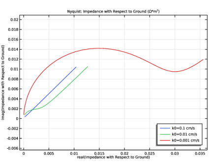
In the Model Builder window, right-click Impedance with Respect to Ground, Real Part (tcd) and choose Duplicate.
2
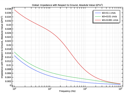
In the Settings window for 1D Plot Group, type Impedance with Respect to Ground, Absolute Value in the Label text field.
Global 1
1
In the Model Builder window, expand the Impedance with Respect to Ground, Absolute Value node, then click Global 1.
2
In the Settings window for Global, locate the y-Axis Data section.
3
Ω*m^2
4
In the Impedance with Respect to Ground, Absolute Value toolbar, click Plot ().
Impedance with Respect to Ground, Phase Angle
1
In the Model Builder window, right-click Impedance with Respect to Ground, Absolute Value and choose Duplicate.
2
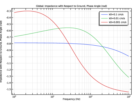
In the Settings window for 1D Plot Group, type Impedance with Respect to Ground, Phase Angle in the Label text field.
Global 1
1
In the Model Builder window, expand the Impedance with Respect to Ground, Phase Angle node, then click Global 1.
2
In the Settings window for Global, locate the y-Axis Data section.
3
4
In the Impedance with Respect to Ground, Phase Angle toolbar, click Plot ().