|
|
|


|
1
|
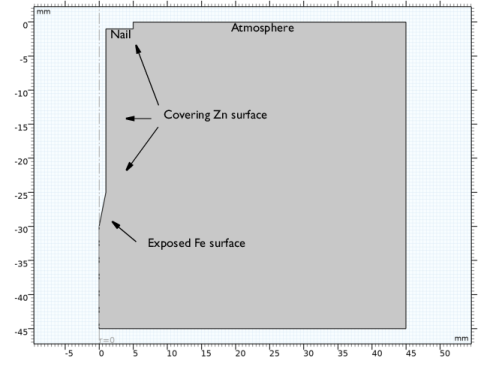
In the Model Wizard window, Make use of symmetry to model the nail using a 2D axisymmetric geometry.
|
|
2
|
|
3
|
In the Select Physics tree, select Electrochemistry>Primary and Secondary Current Distribution>Secondary Current Distribution (cd).
|
|
4
|
Click Add.
|
|
5
|
Click
|
|
6
|
|
7
|
Click
|
|
1
|
|
2
|
|
3
|
|
4
|
Browse to the model’s Application Libraries folder and double-click the file galvanized_nail_parameters.txt.
|
|
1
|
|
2
|
|
3
|
|
1
|
|
2
|
|
3
|
|
4
|
|
1
|
|
2
|
|
4
|
|
1
|
|
2
|
Select the object sq1 only.
|
|
3
|
|
4
|
|
5
|
Select the object pol1 only.
|
|
6
|
|
7
|
|
1
|
|
2
|
|
3
|
|
1
|
|
2
|
|
3
|
|
1
|
|
2
|
|
3
|
|
4
|
|
5
|
|
6
|
Click OK.
|
|
1
|
In the Model Builder window, under Component 1 (comp1)>Secondary Current Distribution (cd) click Electrolyte 1.
|
|
2
|
|
3
|
|
1
|
|
2
|
|
3
|
|
1
|
|
2
|
|
3
|
|
4
|
Locate the Electrode Kinetics section. From the Kinetics expression type list, choose Anodic Tafel equation.
|
|
5
|
|
6
|
|
1
|
|
2
|
|
3
|
|
4
|
Locate the Electrode Kinetics section. From the Kinetics expression type list, choose Cathodic Tafel equation.
|
|
5
|
|
6
|
|
1
|
|
2
|
|
3
|
|
1
|
|
2
|
|
3
|
|
4
|
|
5
|
|
1
|
|
2
|
|
3
|
|
4
|
|
1
|
|
2
|
|
3
|
|
1
|
|
2
|
|
3
|
|
4
|
|
5
|
|
1
|
|
2
|
|
3
|
|
5
|
|
6
|
|
8
|
|
1
|
|
2
|
|
1
|
|
2
|
|
3
|
|
4
|
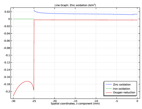
Click Replace Expression in the upper-right corner of the y-Axis Data section. From the menu, choose Component 1 (comp1)>Secondary Current Distribution>Electrode kinetics>cd.iloc_er1 - Local current density - A/m².
|
|
5
|
|
6
|
In the associated text field, type Zinc oxidation.
|
|
7
|
|
8
|
|
9
|
|
10
|
|
11
|
Select the Description check box.
|
|
1
|
|
2
|
|
3
|
|
4
|
|
5
|
|
1
|
|
2
|
|
3
|
|
4
|
Click Replace Expression in the upper-right corner of the y-Axis Data section. From the menu, choose Component 1 (comp1)>Secondary Current Distribution>Electrode kinetics>cd.iloc_er2 - Local current density - A/m².
|
|
5
|
|
1
|
|
2
|
|
3
|
|
1
|
|
2
|
|
3
|
|
4
|
|
5
|
|
1
|
|
2
|
Clear the Convection check box.
|
|
1
|
In the Model Builder window, under Component 1 (comp1)>Transport of Diluted Species (tds) click Transport Properties 1.
|
|
2
|
|
3
|
|
1
|
|
3
|
|
4
|
|
5
|
|
1
|
|
2
|
|
3
|
|
1
|
|
2
|
|
3
|
|
1
|
In the Model Builder window, expand the Electrode Surface Coupling 1 node, then click Reaction Coefficients 1.
|
|
2
|
|
3
|
|
4
|
|
5
|
|
1
|
In the Model Builder window, under Component 1 (comp1)>Transport of Diluted Species (tds) right-click Electrode Surface Coupling 1 and choose Duplicate.
|
|
2
|
|
3
|
|
1
|
In the Model Builder window, expand the Electrode Surface Coupling 2 node, then click Reaction Coefficients 1.
|
|
2
|
|
3
|
|
1
|
In the Model Builder window, under Component 1 (comp1)>Secondary Current Distribution (cd)>Electrode Surface 1 click Oxygen reaction.
|
|
2
|
|
3
|
|
1
|
|
2
|
|
3
|
|
1
|
|
2
|
|
3
|
|
1
|
|
2
|
Click
|
|
1
|
|
2
|
|
1
|
|
2
|
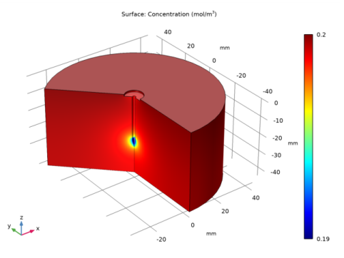
In the Settings window for Surface, click Replace Expression in the upper-right corner of the Expression section. From the menu, choose Component 1 (comp1)>Transport of Diluted Species>Species c>c - Concentration - mol/m³.
|
|
3
|
|
1
|
|
2
|
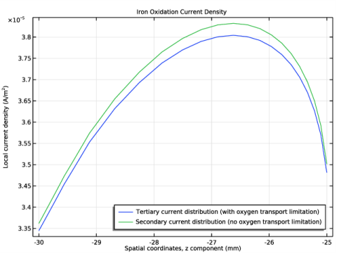
In the Settings window for 1D Plot Group, type Iron Oxidation Current Density in the Label text field.
|
|
1
|
|
2
|
|
3
|
|
4
|
Click Replace Expression in the upper-right corner of the y-Axis Data section. From the menu, choose cd.iloc_er1 - Local current density - A/m².
|
|
5
|
|
6
|
|
7
|
|
8
|
|
9
|
|
1
|
|
2
|
|
3
|
|
4
|
Locate the Legends section. In the table, enter the following settings:
|
|
1
|
|
2
|
|
3
|
|
4
|