|
|
|


|
O2
|
H2
|
||||
|
A/m2
|
7.1·10-5
|
7.7·10-7
|
1.1·10-2
|
||
|
1
|
|
2
|
In the Select Physics tree, select Electrochemistry>Tertiary Current Distribution, Nernst-Planck>Tertiary, Supporting Electrolyte (tcd).
|
|
3
|
Click Add.
|
|
4
|
|
5
|
In the Concentrations table, enter the following settings:
|
|
6
|
Click
|
|
7
|
|
8
|
Click
|
|
1
|
|
2
|
|
3
|
|
4
|
Browse to the model’s Application Libraries folder and double-click the file cathodic_protection_in_concrete_parameters.txt.
|
|
1
|
|
2
|
|
3
|
|
4
|
Click Browse.
|
|
5
|
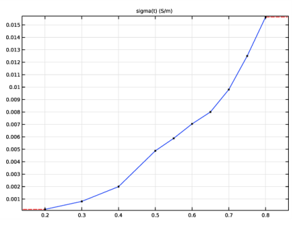
Browse to the model’s Application Libraries folder and double-click the file cathodic_protection_in_concrete_sigma.txt.
|
|
6
|
Click Import.
|
|
7
|
|
8
|
|
9
|
Click
|
|
1
|
|
2
|
|
3
|
|
4
|
Click Browse.
|
|
5
|
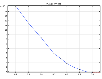
Browse to the model’s Application Libraries folder and double-click the file cathodic_protection_in_concrete_D_O2.txt.
|
|
6
|
Click Import.
|
|
7
|
|
8
|
|
9
|
Click
|
|
1
|
|
2
|
|
3
|
|
4
|
|
5
|
|
6
|
|
1
|
|
2
|
|
3
|
|
4
|
|
5
|
|
6
|
|
1
|
|
2
|
Select the object r1 only.
|
|
3
|
|
4
|
|
5
|
Select the object c1 only.
|
|
6
|
|
1
|
In the Model Builder window, under Component 1 (comp1)>Tertiary Current Distribution, Nernst-Planck (tcd) click Electrolyte 1.
|
|
2
|
|
3
|
|
4
|
Locate the Electrolyte Current Conduction section. From the σl list, choose User defined. In the associated text field, type sigma(PS).
|
|
1
|
|
2
|
|
3
|
|
1
|
|
1
|
|
2
|
|
3
|
|
4
|
Click OK.
|
|
5
|
|
6
|
|
7
|
Locate the Electrode Kinetics section. From the Kinetics expression type list, choose Thermodynamic equilibrium.
|
|
1
|
|
3
|
In the Settings window for Electrode Surface, locate the Electrode Phase Potential Condition section.
|
|
4
|
|
1
|
|
2
|
|
3
|
|
4
|
Click OK.
|
|
5
|
|
6
|
|
7
|
|
8
|
Locate the Equilibrium Potential section. From the Eeq list, choose User defined. In the associated text field, type Eeq_O2.
|
|
9
|
Locate the Electrode Kinetics section. From the Kinetics expression type list, choose Cathodic Tafel equation.
|
|
10
|
|
11
|
|
1
|
|
2
|
|
3
|
|
4
|
|
5
|
Click OK.
|
|
6
|
|
7
|
|
8
|
|
9
|
|
10
|
|
1
|
|
2
|
|
3
|
|
4
|
Click OK.
|
|
5
|
|
6
|
|
7
|
|
8
|
|
9
|
|
1
|
|
3
|
|
4
|
|
5
|
|
1
|
|
2
|
|
3
|
|
1
|
|
2
|
|
3
|
|
4
|
Click
|
|
6
|
|
1
|
|
2
|
|
1
|
|
3
|
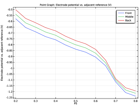
In the Settings window for Point Graph, click Replace Expression in the upper-right corner of the y-Axis Data section. From the menu, choose Component 1 (comp1)>Tertiary Current Distribution, Nernst-Planck>tcd.Evsref - Electrode potential vs. adjacent reference - V.
|
|
4
|
|
5
|
|
7
|
|
1
|
|
2
|
|
1
|
|
2
|
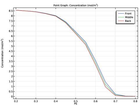
In the Settings window for Point Graph, click Replace Expression in the upper-right corner of the y-Axis Data section. From the menu, choose Component 1 (comp1)>Tertiary Current Distribution, Nernst-Planck>Species c>c - Concentration - mol/m³.
|
|
1
|
|
2
|
In the Settings window for 1D Plot Group, type Oxygen Reduction Current Density in the Label text field.
|
|
1
|
In the Model Builder window, expand the Oxygen Reduction Current Density node, then click Point Graph 1.
|
|
2
|
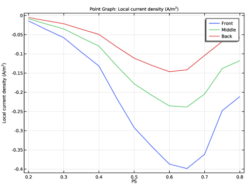
In the Settings window for Point Graph, click Replace Expression in the upper-right corner of the y-Axis Data section. From the menu, choose Component 1 (comp1)>Tertiary Current Distribution, Nernst-Planck>Electrode kinetics>tcd.iloc_er1 - Local current density - A/m².
|
|
1
|
|
2
|
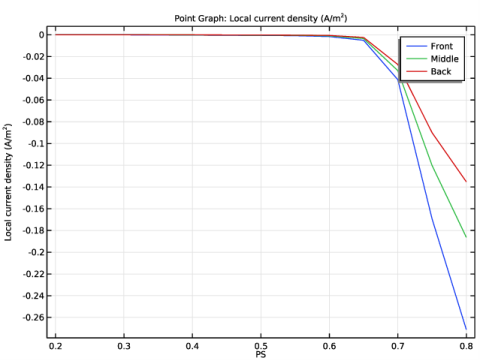
In the Settings window for 1D Plot Group, type Iron Oxidation Current Density in the Label text field.
|
|
1
|
In the Model Builder window, expand the Iron Oxidation Current Density node, then click Point Graph 1.
|
|
2
|
In the Settings window for Point Graph, click Replace Expression in the upper-right corner of the y-Axis Data section. From the menu, choose Component 1 (comp1)>Tertiary Current Distribution, Nernst-Planck>Electrode kinetics>tcd.iloc_er2 - Local current density - A/m².
|
|
3
|
|
1
|
|
2
|
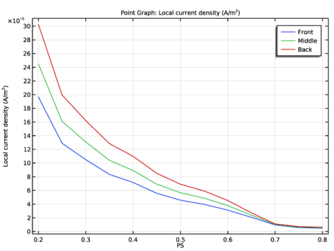
In the Settings window for 1D Plot Group, type Hydrogen Evolution Current Density in the Label text field.
|
|
1
|
In the Model Builder window, expand the Hydrogen Evolution Current Density node, then click Point Graph 1.
|
|
2
|
In the Settings window for Point Graph, click Replace Expression in the upper-right corner of the y-Axis Data section. From the menu, choose Component 1 (comp1)>Tertiary Current Distribution, Nernst-Planck>Electrode kinetics>tcd.iloc_er3 - Local current density - A/m².
|
|
3
|