|
|
|
|
•
|
|
•
|
|
•
|
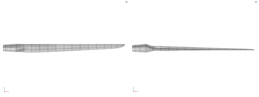
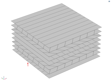
Modeling a composite laminated shell requires a surface geometry (2D), in general called a base surface, and a Layered Material node which adds an extra dimension (1D) to the base surface geometry in the surface normal direction. You can use the Layered Material functionality to model several layers stacked on top of each other having different thicknesses, material properties, and fiber orientations. You can optionally specify the interface materials between the layers and control mesh elements in each layer.
|
|
•
|
From a constitutive model point of view, you use the equivalent single layer (ESL) theory based formulation in Layered Linear Elastic material model of Shell interface.
|
|
1
|
|
2
|
|
3
|
Click Add.
|
|
4
|
Click
|
|
5
|
|
6
|
Click
|
|
1
|
|
2
|
|
1
|
|
2
|
|
3
|
|
4
|
|
5
|
Click Browse.
|
|
6
|
Browse to the model’s Application Libraries folder and double-click the file wind_turbine_composite_blade.mphbin.
|
|
7
|
Click Import.
|
|
1
|
|
2
|
|
3
|
|
5
|
|
1
|
|
2
|
|
3
|
|
5
|
|
1
|
|
2
|
|
3
|
|
5
|
|
1
|
|
2
|
|
3
|
|
4
|
|
5
|
|
1
|
|
2
|
|
3
|
|
1
|
|
2
|
|
3
|
|
1
|
|
2
|
|
1
|
In the Model Builder window, under Global Definitions right-click Materials and choose Blank Material.
|
|
2
|
|
1
|
|
2
|
In the Settings window for Layered Material, type Layered Material: CE-[0]_10 in the Label text field.
|
|
3
|
|
1
|
|
2
|
|
1
|
|
2
|
In the Settings window for Layered Material, type Layered Material: GV-[0_5/45_5/-45_5/90_5]_s in the Label text field.
|
|
3
|
|
4
|
Click
|
|
6
|
Click to expand the Preview Plot Settings section. In the Thickness-to-width ratio text field, type 0.6.
|
|
7
|
Locate the Layer Definition section. Click Layer Stack Preview in the upper-right corner of the section.
|
|
1
|
|
2
|
|
1
|
|
2
|
|
3
|
|
1
|
|
2
|
In the Settings window for Layered Material Link, type Layered Material Link: Glass-Vinylester in the Label text field.
|
|
3
|
Locate the Link Settings section. From the Material list, choose Layered Material: GV-[0_5/45_5/-45_5/90_5]_s (lmat2).
|
|
1
|
|
2
|
In the Settings window for Layered Material Link, type Layered Material Link: PVC Foam in the Label text field.
|
|
3
|
|
1
|
In the Settings window for Layered Material Stack, click to expand the Preview Plot Settings section.
|
|
2
|
|
3
|
Locate the Layered Material Settings section. Click Layer Cross Section Preview in the upper-right corner of the section.
|
|
1
|
In the Model Builder window, under Component 1 (comp1) right-click Shell (shell) and choose Material Models>Layered Linear Elastic Material.
|
|
2
|
|
3
|
|
4
|
|
1
|
In the Model Builder window, under Global Definitions>Materials click Material: Carbon-Epoxy (mat1).
|
|
2
|
|
1
|
|
2
|
|
1
|
|
2
|
|
4
|
|
5
|
In the Show More Options dialog box, in the tree, select the check box for the node Physics>Advanced Physics Options.
|
|
6
|
Click OK.
|
|
1
|
In the Model Builder window, under Component 1 (comp1)>Shell (shell) click Layered Linear Elastic Material 1.
|
|
2
|
In the Settings window for Layered Linear Elastic Material, click to expand the Shear Correction Factor section.
|
|
3
|
|
1
|
|
2
|
|
3
|
|
1
|
|
2
|
|
3
|
|
4
|
|
1
|
In the Model Builder window, under Global Definitions>Load and Constraint Groups click Load Group 1.
|
|
2
|
|
1
|
|
2
|
|
3
|
|
4
|
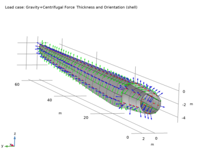
Locate the Rotating Frame section. From the Axis of rotation list, choose User defined. Specify the rbp vector as
|
|
5
|
|
6
|
|
7
|
|
8
|
|
9
|
|
1
|
In the Model Builder window, under Global Definitions>Load and Constraint Groups click Load Group 2.
|
|
2
|
|
1
|
|
2
|
|
3
|
|
1
|
|
2
|
|
3
|
|
4
|
|
6
|
|
1
|
|
2
|
|
1
|
|
2
|
|
3
|
|
4
|
Click
|
|
6
|
|
1
|
In the Model Builder window, expand the Layered Materials node, then click Layered Material 2 (Shell Geometry).
|
|
2
|
|
3
|
|
1
|
|
2
|
|
3
|
|
1
|
|
2
|
|
3
|
|
4
|
|
1
|
|
2
|
|
4
|
Locate the Expressions section. In the table, enter the following settings:
|
|
5
|
Click
|
|
1
|
|
2
|
|
3
|
|
4
|
Locate the Expressions section. In the table, enter the following settings:
|
|
5
|
Click
|
|
1
|
|
2
|
|
3
|
|
4
|
|
1
|
|
2
|
|
3
|
|
4
|
|
5
|
|
1
|
|
2
|
|
3
|
|
1
|
|
2
|
|
3
|
|
4
|
|
1
|
|
2
|
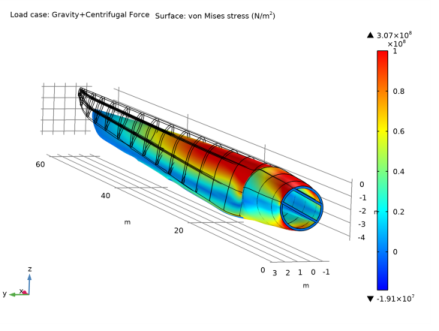
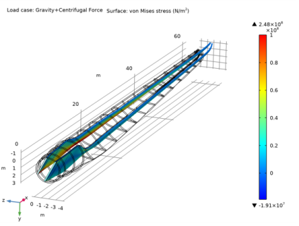
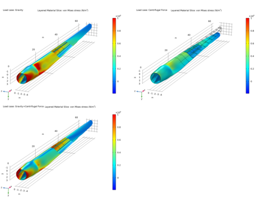
In the Settings window for 3D Plot Group, type Stress, Slice (Carbon-Epoxy) in the Label text field.
|
|
3
|
|
1
|
In the Model Builder window, expand the Results>Stress, Slice (Carbon-Epoxy)>Layered Material Slice 1 node, then click Layered Material Slice 1.
|
|
2
|
|
3
|
|
4
|
|
5
|
|
6
|
|
1
|
|
2
|
|
3
|
|
4
|
|
1
|
|
2
|
|
3
|
|
4
|
In the Local z-coordinate text field, type 5*th, 17*th, 30*th, 50*th+0.5*thc, 70*th+thc, 83*th+thc, 95*th+thc.
|
|
5
|
|
6
|
|
7
|
|
8
|
|
1
|
|
2
|
|
3
|
|
5
|
|
6
|
|
1
|
|
2
|
|
1
|
|
2
|
|
3
|
|
4
|
|
5
|
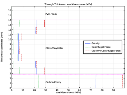
In the associated text field, type von Mises stress (MPa).
|
|
6
|
|
7
|
In the associated text field, type Thickness coordinate (mm).
|
|
8
|
|
9
|
|
10
|
|
11
|
|
12
|
|
13
|
|
1
|
In the Model Builder window, expand the Stress, Through Thickness (shell) node, then click Through Thickness 1.
|
|
2
|
|
3
|
|
5
|
|
6
|
|
7
|
|
8
|
|
9
|
Find the Interface positions subsection. From the Show interface positions list, choose Interfaces between layered materials.
|
|
10
|
Click to expand the Coloring and Style section. Find the Line style subsection. From the Line list, choose Cycle.
|
|
11
|
|
1
|
|
2
|
|
3
|
|
5
|
|
6
|
|
1
|
|
2
|
|
1
|
|
2
|
|
3
|
|
1
|
|
2
|
|
1
|
|
2
|
|
3
|
|
4
|
|
5
|
|
1
|
|
2
|
|
3
|
Find the Studies subsection. In the Select Study tree, select Preset Studies for Selected Physics Interfaces>Eigenfrequency, Prestressed.
|
|
4
|
|
5
|
|
1
|
|
2
|
|
1
|
|
2
|
|
3
|
Click
|
|
1
|
|
2
|
|
3
|
|
4
|
Click
|
|
1
|
|
2
|
|
3
|
|
5
|
|
6
|
|
1
|
In the Model Builder window, expand the Layered Materials 1 node, then click Layered Material 6 (Shell Geometry).
|
|
2
|
|
3
|
|
1
|
|
2
|
|
3
|
|
1
|
|
2
|
|
3
|
|
4
|
|
5
|
|
6
|
|
7
|
|
1
|
|
2
|
|
3
|
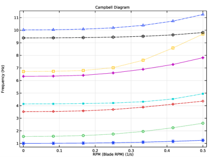
Locate the Data section. From the Dataset list, choose Study: Eigenfrequency/Parametric Solutions 1 (sol4).
|
|
4
|
|
5
|
|
6
|
In the associated text field, type Frequency (Hz).
|
|
7
|
|
1
|
|
2
|
|
4
|
|
5
|
Click to expand the Coloring and Style section. Find the Line style subsection. From the Line list, choose Cycle.
|
|
6
|
|
7
|
|
1
|
|
2
|
|
3
|
|
4
|
|
5
|
|
6
|