You are viewing the documentation for an older COMSOL version. The latest version is available here.
PDF

Material Characteristics of Laminated Composite Shell
Introduction
This model serves the purpose of validation and verification of the Layered Linear Elastic Material model in the Shell interface.
Analysis of laminated composite shells is commonly based on one of three different theories (Ref. 1),
1
a
b
c
2
a
b
3
In COMSOL Multiphysics, composites are analyzed either based on Layerwise 3D elasticity theory through the Layered Shell interface or based on FSDT-ESL theory through the Shell interface.
The First Order Shear Deformation Theory (FSDT-ESL) is implemented in the Layered Linear Elastic Material model in the Shell interface available with the Composite Materials Module. This theory treats a heterogeneous laminated composite as a statically equivalent single layer. ESL theory reduces a 3D continuum problem to an equivalent 2D problem, thus reducing the size and computational time of the problem.
This example is a NAFEMS benchmark, described in Benchmarks for Membrane and Bending Analysis of Laminated Shells, Part 2: Stiffness Matrix and Thermal Characteristics (Ref. 2). Membrane and bending stiffness, flexibility matrices, midplane strains in case of unit loading, and the response to a unit change in temperature and unit temperature gradient are verified.
Model Definition
The geometry of the problem consists of eight square layers stacked above each other. The side length is 1 cm and each layer has a thickness of 0.1 mm, as shown in Figure 2. The laminate has [0/60/-60/0]s stacking sequence as shown in Figure 1.
Figure 1: Stacking sequence [0/60/-60/0]s from bottom to top, showing fiber orientation in each ply.
Figure 2: Cross-section view of laminated composite shell showing thickness (0.1mm) of each ply.
Material Properties
The orthotropic material properties (Young’s modulus, shear modulus, Poisson’s ratio, and thermal expansion coefficients) are given in Table 1:
{E1,E2,E3}
{G12,G23,G13}
{υ12,υ23,υ13}
{α1,α2,α3}
All material properties are given in the layer coordinate system (local material directions of a layer), where the first axis is aligned with the fiber orientation.
Boundary Conditions
The constraints and loads applied on each node for unit loading and thermal loading are given in the tables below.
N1
N2
N12
M1
M2
M12
u, v, w,θx, θy, θz
u, v, w, θx, θy, θz
u, v, w, θx, θy, θz
u, v, w, θx, θy, θz
u, v, w, θx, θy, θz
u, v, w, θy, θz
u, v, w, θz
u, θz
θz
v, θz
u, θz
θz
w, θz
u, w, θz
θz
v, θz
u, θz
θz
v, θz
θz
w, θz
θz
θz
θz
θz
θz
v, θz
θz
 
N1
N2
N12
M1
M2
M12
My=-5e-3
Mx=5e-3
Fy=5e-3
Fx=5e-3
My=-5e-3
Mx=-5e-3
Fx=5e-3
Fy=5e-3
My=5e-3
Mx=5e-3
Fz=2
Fx=5e-3
Fy=5e-3
Fx=5e-3
Fy=5e-3
My=5e-3
Mx=-5e-3
Fz=-2
Note that the way the benchmark is specified, it is assumed that a single first-order four-node element is used. This is the only case when such a specification can give a homogeneous strain state.
The node numbers specified in the benchmark are equal to the point numbers in the COMSOL Multiphysics geometry. The signs of the point loads and moments are adjusted to give positive unit loads and moments as specified in Ref. 2. The rotation around the z-axis, θz, is automatically constrained so it does not need to be considered. The unit change in temperature and unit temperature gradient is prescribed using a Thermal Expansion subnode of the Layered Linear Elastic Material.
Results and Discussion
The results presented in the benchmark (Ref. 2) are for the Classical Laminated Plate Theory (CLPT-ESL). The implementation of Layered Linear Elastic Model is however based on First Order Shear Deformation Theory (FSDT-ESL). The difference between both theories is that FSDT theory considers transverse shear stresses, but for the benchmark example with unit in-plane loading, the results should match between both theories because of the zero or negligible shear strains. Note that the bending strains are actually curvatures, but for consistency purpose they will be called as strains throughout this document.
The relation between in-plane forces and moments with midplane strains is represented by
(1)
where A, B, and D are called extensional stiffness matrix, bending-extensional stiffness matrix, and bending stiffness matrix, respectively.
The same relation can be represented on flexibility form as
(2)
where a, b, and d are called extensional flexibility matrix, bending-extensional flexibility matrix, and bending flexibility matrix, respectively. The relationship between stiffness and flexibility matrices is
(3)
In the benchmark, the laminate flexibility matrix are computed in two ways, first directly from CLPT theory and then from midplane strains when unit loads and moments are applied. When unit in-plane forces Nij and unit moments Mij are applied, the midplane strains and curvature are the elements of flexibility matrix. The midplane strains in the benchmark are computed numerically using commercial finite element software. Table 4 and Table 5 shows the flexibility matrix from the benchmark (Ref. 2).
N1
N2
N12
M1
M2
M12
γ12
κ12
N1
N2
N12
M1
M2
M12
γ12
κ12
The midplane strains for a unit change in temperature are given in the benchmark (Ref. 2)
γ12
κ12
The midplane strains for a unit temperature gradient are given in the benchmark (Ref. 2)
γ12
κ12
In COMSOL Multiphysics, the stiffness (A, B, D) and flexibility matrices (a, b, d) are available as postprocessing variables. The midplane strains are computed for each unit load cases (six load cases). The strain vector then represents a column in the full flexibility matrix for a unit load case. For example, the membrane and bending midplane strains forms a first column of full flexibility matrix for unit N1. The full flexibility matrix based on First Order Shear Deformation Theory (FSDT-ESL) and midplane strains from COMSOL are shown in Table 8 and Table 9 below
N1
N2
N12
M1
M2
M12
γ12
κ12
 
N1
N2
N12
M1
M2
M12
γ12
κ12
The midplane strains for unit change in temperature and unit temperature gradient from COMSOL are
γ12
κ12
 
γ12
κ12
When comparing Table 4 to Table 8, Table 5 to Table 9, Table 6 to Table 10, and Table 7 to Table 11, an exact match can be found between the results of benchmark model and the results computed in COMSOL Multiphysics. The full flexibility matrix is found by inverting the full stiffness matrix, so the verification of the full flexibility matrix automatically verifies also the correctness of full stiffness matrix (not presented here but shown in the model).
Notes About the COMSOL Implementation
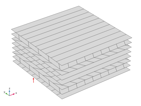
Modeling a composite laminated shell requires a surface geometry (2D), in general called a base surface, and a Layered Material node which adds an extra dimension (1D) to the base surface geometry in the surface normal direction. In the Layered Material node, you can model many layers stacked on top of each other having different thickness, material properties, and fiber orientations. You can also optionally specify the interface materials between the layers and control mesh elements in each layer.
The Layered Material Link and Layered Material Stack have an option to transform given Layered Material into a symmetric or antisymmetric laminate. A repeated laminate can also be constructed using a transform option.
From a constitutive equations point of view, you can either use the Layerwise (LW) theory based Layered Shell interface, or Equivalent Single Layer (ESL) theory based Layered Linear Elastic Material node in the Shell interface.
The six different unit load cases and two thermal loading cases requires different boundary conditions and point loads as shown in Table 2 and Table 3. To solve all these cases in a single study, different load groups and constraint groups are created, and constrains and loads corresponding to a particular case are assigned to these groups according to Table 2 and Table 3. In the Stationary node in the study, appropriate load and constraint groups are selected for each load case.
References
1. J. N. Reddy, Mechanics of Laminated Composite Plates and Shells: Theory and Analysis, Second Edition, CRC Press, 2004.
2. P. Hopkins, Benchmarks for Membrane and Bending Analysis of Laminated Shells, Part 1: Stiffness Matrix and Thermal Characteristics, NAFEMS, 2005.
Application Library path: Composite_Materials_Module/Verification_Examples/laminated_shell_material_characteristics
Modeling Instructions
From the File menu, choose New.
New
In the New window, click  Model Wizard.
Model Wizard
1
In the Model Wizard window, click  3D.
2
In the Select Physics tree, select Structural Mechanics>Shell (shell).
3
Click Add.
4
Click  Study.
5
In the Select Study tree, select General Studies>Stationary.
6
Global Definitions
Parameters 1
Load the material properties from a file.
1
In the Model Builder window, under Global Definitions click Parameters 1.
2
In the Settings window for Parameters, locate the Parameters section.
3
Click  Load from File.
4
Browse to the model’s Application Libraries folder and double-click the file laminated_shell_material_characteristics_parameters.txt.
In order to apply unit in-plane forces and moments, as well as unit temperature difference and unit temperature gradient, create separate load and constraint groups.
Load Group for Unit N1
1
In the Model Builder window, right-click Global Definitions and choose Load and Constraint Groups>Load Group.
2
In the Settings window for Load Group, type Load Group for Unit N1 in the Label text field.
3
4
Load Groups for Unit Loading
1
In the Model Builder window, under Global Definitions>Load and Constraint Groups click Group 1.
2
In the Settings window for Group, type Load Groups for Unit Loading in the Label text field.
Load Group for Unit Temperature Difference
1
In the Model Builder window, right-click Load and Constraint Groups and choose Load Group.
2
In the Settings window for Load Group, type Load Group for Unit Temperature Difference in the Label text field.
Load Group for Unit Temperature Gradient
1
Right-click Load and Constraint Groups and choose Load Group.
2
In the Settings window for Load Group, type Load Group for Unit Temperature Gradient in the Label text field.
3
Load Groups for Thermal Loading
1
In the Model Builder window, under Global Definitions>Load and Constraint Groups click Group 2.
2
In the Settings window for Group, type Load Groups for Thermal Loading in the Label text field.
Constraint Group for Unit N1, N2, N12, M1 and M2
1
In the Model Builder window, right-click Load and Constraint Groups and choose Constraint Group.
2
In the Settings window for Constraint Group, type Constraint Group for Unit N1, N2, N12, M1 and M2 in the Label text field.
3
4
Constraint Groups for Unit Loading
1
In the Model Builder window, under Global Definitions>Load and Constraint Groups click Group 3.
2
In the Settings window for Group, type Constraint Groups for Unit Loading in the Label text field.
Constraint Group for Thermal Loading
1
In the Model Builder window, right-click Load and Constraint Groups and choose Constraint Group.
2
In the Settings window for Constraint Group, type Constraint Group for Thermal Loading in the Label text field.
Material 1 (mat1)
In the Model Builder window, right-click Materials and choose Blank Material.
Now add a Layered Material node and assign appropriate thickness and rotation angles to each layer. The laminate is symmetric. It is sufficient to define only half the laminate in the Layered Material node. The transformation into a full laminate is performed through the layered material settings in the Layered Material Link node.
Layered Material: [0/60/-60/0]_s
1
Right-click Materials and choose Layered Material.
2
In the Settings window for Layered Material, locate the Layer Definition section.
3
4
Click Add three times.
5
6
In the Label text field, type Layered Material: [0/60/-60/0]_s.
Geometry 1
Work Plane 1 (wp1)
In the Geometry toolbar, click  Work Plane.
Work Plane 1 (wp1)>Plane Geometry
In the Model Builder window, click Plane Geometry.
Work Plane 1 (wp1)>Square 1 (sq1)
1
In the Work Plane toolbar, click  Square.
2
In the Settings window for Square, locate the Size section.
3
In the Side length text field, type 1e-2.
4
Click  Build Selected.
5
Click the  Zoom Extents button in the Graphics toolbar.
Materials
Layered Material Link 1 (llmat1)
1
In the Model Builder window, under Component 1 (comp1) right-click Materials and choose Layers>Layered Material Link.
The half laminate defined in the Layered Material node can be transformed into a full symmetric laminate using a transform option in the layered material settings.
2
In the Settings window for Layered Material Link, locate the Layered Material Settings section.
3
From the Transform list, choose Symmetric.
4
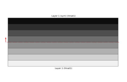
Click to expand the Preview Plot Settings section. In the Thickness-to-width ratio text field, type 0.5.
5
Locate the Layered Material Settings section. Click Layer Cross Section Preview in the upper-right corner of the section.
6
Click Layer Stack Preview in the upper-right corner of the Layered Material Settings section.
The geometry is in an XY-plane in which the fibers are oriented with respect to the X direction. Hence set the first axis of the laminate coordinate system in the X direction.
Definitions (comp1)
Boundary System 1 (sys1)
1
In the Model Builder window, expand the Component 1 (comp1)>Definitions node, then click Boundary System 1 (sys1).
2
In the Settings window for Boundary System, locate the Settings section.
3
Find the Coordinate names subsection. From the Axis list, choose x.
Shell (shell)
1
Click the  Show More Options button in the Model Builder toolbar.
2
In the Show More Options dialog box, in the tree, select the check box for the node Physics>Advanced Physics Options.
3
Set the discretization for the displacement field to Linear in order to resemble the benchmark example.
4
In the Model Builder window, under Component 1 (comp1) click Shell (shell).
5
In the Settings window for Shell, click to expand the Discretization section.
6
From the Displacement field list, choose Linear.
Layered Linear Elastic Material 1
1
In the Physics toolbar, click  Boundaries and choose Layered Linear Elastic Material.
In order to study two thermal load cases separately, add two Thermal Expansion subfeatures and activate them in different load groups.
2
3
In the Settings window for Layered Linear Elastic Material, locate the Linear Elastic Material section.
4
From the Solid model list, choose Orthotropic.
Thermal Expansion for Unit Temperature Difference
1
In the Physics toolbar, click  Attributes and choose Thermal Expansion.
2
In the Settings window for Thermal Expansion, type Thermal Expansion for Unit Temperature Difference in the Label text field.
3
Locate the Model Input section. From the T list, choose User defined. In the associated text field, type 293.15[K] +1[K].
4
In the Physics toolbar, click  Load Group and choose Load Group for Unit Temperature Difference.
Layered Linear Elastic Material 1
In the Model Builder window, click Layered Linear Elastic Material 1.
Thermal Expansion for Unit Temperature Gradient
1
In the Physics toolbar, click  Attributes and choose Thermal Expansion.
2
In the Settings window for Thermal Expansion, type Thermal Expansion for Unit Temperature Gradient in the Label text field.
3
Locate the Thermal Bending section. From the list, choose Temperature gradient in thickness direction.
4
In the T text field, type 1[K/m].
5
In the Physics toolbar, click  Load Group and choose Load Group for Unit Temperature Gradient.
Global Definitions
Material 1 (mat1)
1
In the Model Builder window, under Global Definitions>Materials click Material 1 (mat1).
2
In the Settings window for Material, locate the Material Contents section.
3
Apply different constraints and point loads for different load cases as shown in Table 2 and Table 3. Attach appropriate load and constraint groups to these constraints and load features.
Shell (shell)
Fixed Constraint for Unit N1, N2, N12, M1 and M2
1
In the Physics toolbar, click  Points and choose Fixed Constraint.
2
In the Settings window for Fixed Constraint, type Fixed Constraint for Unit N1, N2, N12, M1 and M2 in the Label text field.
3
4
In the Physics toolbar, click  Constraint Group and choose Constraint Group for Unit N1, N2, N12, M1 and M2.
Prescribed Displacement/Rotation for Unit N1 and M1
1
In the Physics toolbar, click  Points and choose Prescribed Displacement/Rotation.
2
In the Settings window for Prescribed Displacement/Rotation, type Prescribed Displacement/Rotation for Unit N1 and M1 in the Label text field.
3
4
Locate the Prescribed Displacement section. Select the Prescribed in x direction check box.
5
In the Physics toolbar, click  Constraint Group and choose Constraint Group for Unit N1 and M1.
6
Duplicate the Prescribed Displacement/Rotation 1 node nine times to get required numbers of nodal constraints. Label, selection, constraints, constraint groups should be as shown in table below.
Point Load for Unit N1
1
In the Physics toolbar, click  Points and choose Point Load.
2
In the Settings window for Point Load, type Point Load for Unit N1 in the Label text field.
3
4
Locate the Force section. Specify the FP vector as
5
In the Physics toolbar, click  Load Group and choose Load Group: Gravity.
6
Duplicate the Point Load 1 node nine times to get required numbers of nodal loads. Label, selection, loads, load groups should be as shown in the table below.
Mesh 1
Use a single quadrilateral element.
Mapped 1
1
In the Mesh toolbar, click  Boundary and choose Mapped.
2
In the Settings window for Mapped, locate the Boundary Selection section.
3
From the Selection list, choose All boundaries.
Distribution 1
1
Right-click Mapped 1 and choose Distribution.
2
In the Settings window for Distribution, locate the Edge Selection section.
3
From the Selection list, choose All edges.
4
Locate the Distribution section. In the Number of elements text field, type 1.
5
Click  Build All.
Create eight different load cases each for six unit loads/moments and two for thermal loading. Assign appropriate load groups and constraint groups for each load cases as per Table 2 and Table 3.
Study 1
Disable the default plots for this study.
1
In the Model Builder window, click Study 1.
2
In the Settings window for Study, locate the Study Settings section.
3
Clear the Generate default plots check box.
Step 1: Stationary
1
In the Model Builder window, under Study 1 click Step 1: Stationary.
2
In the Settings window for Stationary, click to expand the Study Extensions section.
3
Select the Define load cases check box.
4
Click  Add seven times.
5
6
In the Home toolbar, click  Compute.
In order to find the laminate flexibility and stiffness matrices, use Point Matrix Evaluation node under Evaluation Group.
Results
Extensional Flexibility Matrix
1
In the Results toolbar, click  Evaluation Group.
2
In the Settings window for Evaluation Group, locate the Data section.
3
From the Parameter selection (Load case) list, choose First.
4
Click to expand the Format section. From the Include parameters list, choose Off.
5
In the Label text field, type Extensional Flexibility Matrix.
Point Matrix Evaluation 1
1
In the Extensional Flexibility Matrix toolbar, click  More Evaluations and choose Point Matrix Evaluation.
2
3
In the Settings window for Point Matrix Evaluation, click Replace Expression in the upper-right corner of the Expression section. From the menu, choose Component 1 (comp1)>Shell>Stiffness and flexibility>Extensional flexibility matrix>shell.Da - Extensional flexibility matrix - s²/kg.
Extensional Flexibility Matrix
1
In the Model Builder window, click Extensional Flexibility Matrix.
2
In the Extensional Flexibility Matrix toolbar, click  Evaluate.
Table
1
Go to the Table window.
2
Use a Point Evaluation node under Evaluation Group to compute the midplane strains for each load case. The choice of point does not matter as the model gives a uniform strain field.
While evaluating the midplane strains corresponding to each load case, evaluate the corresponding in-plane force or moment postprocessing variable in order to verify the correctness of the applied forces and constraints.
Results
Layered Material 1
In the Results toolbar, click  More Datasets and choose Layered Material.
Cut Point 3D 1
1
In the Results toolbar, click  Cut Point 3D.
2
In the Settings window for Cut Point 3D, locate the Data section.
3
From the Dataset list, choose Layered Material 1.
4
Locate the Point Data section. In the x text field, type 1e-2.
5
In the y text field, type 0.
6
In the z text field, type 0.
Midplane Strains for Unit N1
1
In the Results toolbar, click  Evaluation Group.
2
In the Settings window for Evaluation Group, type Midplane Strains for Unit N1 in the Label text field.
3
Locate the Data section. From the Dataset list, choose Cut Point 3D 1.
4
From the Parameter selection (Load case) list, choose From list.
5
In the Load cases list, select Load case for unit N1.
6
Locate the Format section. From the Include parameters list, choose Off.
Point Evaluation 1
1
Right-click Midplane Strains for Unit N1 and choose Point Evaluation.
2
In the Settings window for Point Evaluation, locate the Expressions section.
3
Midplane Strains for Unit N1
1
In the Model Builder window, click Midplane Strains for Unit N1.
2
In the Midplane Strains for Unit N1 toolbar, click  Evaluate.
Table
1
Go to the Table window.
2
To compute the midplane strains for remaining load cases, duplicate the above node seven times and change the load case in the Data section of corresponding Evaluation Group node. Replace the in-plane force/moment variable in the last row of table in Point Evaluation node with appropriate variable corresponding to the load cases.