PDF

Failure Prediction in a Laminated Composite Shell
Introduction
Laminated composite shells made of carbon fiber reinforced plastics (CFRP) are common in a large variety of applications due to their high strength to weight ratio. Evaluation of the structural integrity of a laminated composite shell for a set of applied loads is necessary to make the design of such structures reliable.
This example shows how to model laminated composite shells using the Layered Linear Elastic Material model in the Shell interface available with the Composite Materials Module.
The structural integrity of a laminate with different fiber orientations in each ply is assessed through the parameters called Failure Index and Safety Factor, using different polynomial failure criteria. Because of the orientation, each ply will have different stiffness in the longitudinal and transverse directions, and hence different response to the loading. The analysis using a polynomial failure criterion is termed first ply failure analysis, where failure in any ply is considered as failure of the whole laminate. In this example, seven different polynomial criteria are compared.
This model is a NAFEMS benchmark model, described in Benchmarks for Membrane and Bending Analysis of Laminated Shells, Part 2: Strength Analysis (Ref. 1). The COMSOL Multiphysics solutions are compared with the reference data.
Model Definition
The physical geometry of the problem consists of four stacked square plies/layers. The side length is 1 cm and each layer has a thickness of 0.05 mm as shown in Figure 2. The laminate is subjected to an in-plane axial tensile load and has a [90/-45/45/0] stacking sequence as shown in Figure 1.
Figure 1: Stacking sequence [90/-45/45/0] of the shell, from bottom to top, showing the fiber orientation in each ply.
Figure 2: Cross-section view of the shell, showing the thickness (0.05 mm) of each ply.
Material Properties
The orthotropic material properties (Young’s modulus, shear modulus, and Poisson’s ratio) are given in Table 1.
{E1,E2,E3}
{G12,G23,G13}
{υ12,υ23,υ13}
The tensile, compressive, and shear strengths are given in Table 2.
{σts1,σts2,σts3}
{σcs1,σcs2,σcs3}
{σss23,σss13,σss12}
All material properties and strengths are given in the layer coordinate system (local material directions of a ply), where the first axis is aligned with the fiber orientation. The local stresses are also evaluated in the layer coordinate system.
Boundary Conditions
The constraints and loads applied on each node of the laminate are given in the table below.
u, v, w,
θx, θy, θz
θz
u, θz
The numbers within parentheses are point numbers in the COMSOL Multiphysics geometry. The boundary conditions provided in the benchmark specifications are applied to the laminated composite shell as a single entity. The rotation around the z-axis, θz, is automatically constrained so it does not need to be considered.
It should be noted that since two point loads are prescribed at nodes, this benchmark can only be run with a single first-order element. This is the only case when such a specification can give a homogeneous stress state.
Failure Criteria
Seven different failure criteria are used to predict failure in the shell. These are the Tsai-Wu Anisotropic, Tsai-Wu Orthotropic, Tsai-Hill, Hoffman, Modified Tsai-Hill, Azzi-Tsai-Hill, and Norris criteria.
Tsai-Wu Anisotropic
For the Tsai-Wu anisotropic criterion, the material strength parameters are taken from Table 2 in order to obtain the same results as with the Tsai-Wu orthotropic criterion. This exercise is done in order to verify the correctness of the implementation. The nonzero elements in the second rank tensor f are given below. Here, and in the following equations, repeated indices do not imply summation.
(1)
The nonzero elements in the fourth rank tensor F, expressed on compacted 6-by-6 form, are
(2)
Modified Tsai-Hill
The Hill criterion in Ref. 1 is called the Modified Tsai-Hill criterion in COMSOL Multiphysics.
Ref. 1 does not give results for either the Tsai-Wu anisotropic, Tsai-Hill, Azzi-Tsai-Hill, nor Norris criteria; so the analytical results for failure index and safety factor are here derived from the stress values given in Ref. 1.
The stresses from Ref. 1 are given in Table 4. Apart from σ11, σ22, and σ12, all other stress components are either zero or negligible.
σ11 (MPa)
σ22 (MPa)
σ12 (MPa)
For all the selected polynomial criteria, the failure index (FI) is written as
(3)
where σi is the 6-by-1 stress vector (sorted using Voigt notation), Fij is a 6-by-6 symmetric matrix (fourth rank tensor) that contains the coefficients for the quadratic terms, and fi is a 6-by-1 vector (second rank tensor) that contains the linear terms. A failure index equal to or greater than 1.0 indicates failure in the material. In order to find the safety factor (SF), the applied stress in Equation 3 is multiplied by the safety factor SF, and the failure index FI is set equal to 1.0, which results in a quadratic equation of the form
(4)
where and .
The lowest positive root in Equation 4 is selected as the safety factor (SF). Based on the stress values given in Table 4, the failure index and safety factor are computed for the criteria for which results in Ref. 1 are missing.
Tsai-Wu Anisotropic
For the Tsai-Wu anisotropic criterion, the nonzero elements of the vector fi and the matrix Fij are given by Equation 1 and Equation 2. By taking values of stresses from Table 4, the failure index and safety factor are computed from Equation 3 and Equation 4, and given in Table 5 below.
Tsai-Hill
For the Tsai-Hill criterion, all elements of the vector fi are zero, while the nonzero elements of the matrix Fij are given by the Equation 5.
(5)
By taking values of stresses from Table 4, the failure index and safety factor are computed from Equation 3, Equation 4 and Equation 5, and given in Table 6 below.
Azzi-Tsai-Hill
For the Azzi-Tsai-Hill criterion, all elements of the vector fi are zero, while the nonzero elements of the matrix Fij are given by Equation 6.
(6)
By taking values of the stresses from Table 4, the failure index and safety factor are computed from Equation 3, Equation 4 and Equation 6, and given in Table 7 below.
Norris
For the Norris criterion, all elements of the vector fi are zero, while the nonzero elements of the matrix Fij are given by Equation 7.
(7)
By taking values of the stresses from Table 4, the failure index and safety factor are computed from Equation 3, Equation 4 and Equation 7, and given in Table 8 below.
Note that for the current model, failure index, safety factor and stresses are computed at the midplane of each ply.
Results and Discussion
The computed stresses are shown in Table 4, while Table 5 to Table 8 show the analytical values for failure index and safety factor (reserve factor) for certain failure criteria. For the Tsai-Wu orthotropic, Modified Tsai-Hill, and Hoffman criteria, the failure index and safety factor are taken from Ref. 1. The results are compared with results from COMSOL Multiphysics.
σ11 from benchmark
σ11, computed
σ22 from benchmark
σ22, computed
σ12 from benchmark
σ12, computed
 
For many industrial and real life applications, the safety factor (SF) is more useful than the failure index (FI). The safety factor (or reserve factor) gives a direct indication of how close the component is to failure. Figure 3 shows the Hoffman safety factor (SF) at the midplane for the different plies. Ply 1 (90 degree ply) is close to failure as expected because of its orientation, where fibers are perpendicular to the loading direction. The von Mises stresses in all plies are shown in Figure 4. The stress in ply 1 is the lowest, but still this layer is still more susceptible to failure due to the orientation of its fibers.
Figure 3: Hoffman safety factors at ply midplanes for the laminated composite shell.
Figure 4: von Mises stress at ply midplanes for the laminated composite shell.
The distribution of the von Mises equivalent stress across the laminate is shown in the Figure 5. The interface between ply 2-ply 3 and ply 3-ply 4 experiences the maximum stresses due to bending of the laminate.
Figure 5: von Mises stress in the laminated composite shell.
The variation of the von Mises stress across the thickness at the middle of the laminate is shown in the Figure 6. It is evident that the von Mises stress is not continuous across the plies. The maximum Mises stress observed about 28-30 MPa in the third and fourth ply, which can be seen in Figure 5. The maximum stress observed at the bottom interface of the two top layers is caused by the bending of the laminate.
Figure 6: Through thickness variation of von Mises stress at the center of the laminated composite shell.
Notes About the COMSOL Implementation
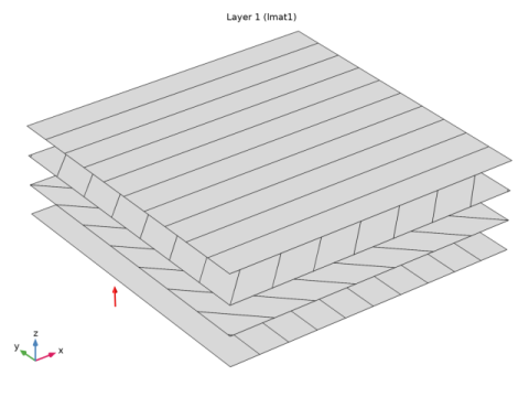
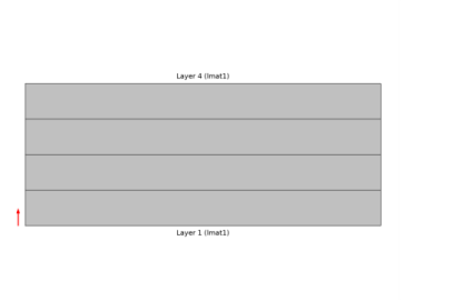
Modeling a composite laminated shell requires a surface geometry (2D), in general called a base surface, and a Layered Material node which adds an extra dimension (1D) to the base surface geometry in the surface normal direction. In the Layered Material node, you can model many layers stacked on top of each other having different thickness, material properties, and fiber orientations. You can also optionally specify the interface materials between the layers and control mesh elements in each layer.
From a constitutive equations point of view, you can either use the Layerwise (LW) theory based Layered Shell interface, or the Equivalent Single Layer (ESL) theory based Layered Linear Elastic Material node in the Shell interface.
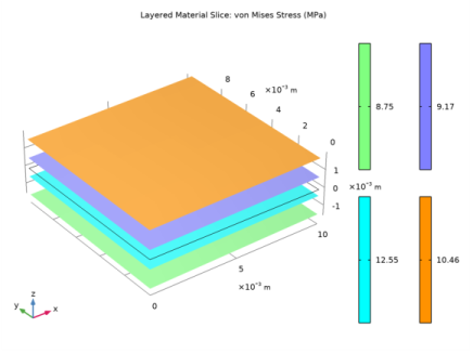
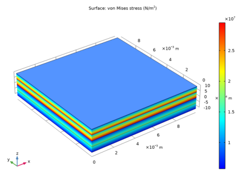
To analyze the results in a composite shell, you can either create slice plot using a Layered Material Slice plot in order to see the in-plane variation of a quantity, or you can create a Through Thickness plot to see the out-of-plane variation of a quantity. In order to visualize the results as a 3D solid object, you can use the Layered Material dataset which creates a virtual 3D solid object combining a surface geometry (2D) and the extra dimension (1D).
Reference
1. P. Hopkins, Benchmarks for Membrane and Bending Analysis of Laminated Shells, Part 2: Strength Analysis, NAFEMS, 2005.
Application Library path: Composite_Materials_Module/Verification_Examples/failure_prediction_in_a_laminated_composite_shell
Modeling Instructions
From the File menu, choose New.
New
In the New window, click  Model Wizard.
Model Wizard
1
In the Model Wizard window, click  3D.
2
In the Select Physics tree, select Structural Mechanics>Shell (shell).
3
Click Add.
4
Click  Study.
5
In the Select Study tree, select General Studies>Stationary.
6
Global Definitions
Parameters 1
Load the material properties and material strengths from a file.
1
In the Model Builder window, under Global Definitions click Parameters 1.
2
In the Settings window for Parameters, locate the Parameters section.
3
Click  Load from File.
4
Browse to the model’s Application Libraries folder and double-click the file failure_prediction_in_a_laminated_composite_shell_materialproperties.txt.
Material 1 (mat1)
1
In the Model Builder window, right-click Materials and choose Blank Material.
Add a Layered Material node and assign appropriate thickness and rotation angles to each ply.
Layered Material: [90/-45/45/0]
1
Right-click Materials and choose Layered Material.
2
In the Settings window for Layered Material, locate the Layer Definition section.
3
4
Click Add three times.
5
6
In the Label text field, type Layered Material: [90/-45/45/0].
7
Locate the Layer Definition section. Click Layer Cross Section Preview in the upper-right corner of the section.
8
Click to expand the Preview Plot Settings section. In the Thickness-to-width ratio text field, type 0.4.
9
Click the  Show Grid button in the Graphics toolbar.
10
Locate the Layer Definition section. Click Layer Cross Section Preview in the upper-right corner of the section.
11
Click Layer Stack Preview in the upper-right corner of the Layer Definition section.
Geometry 1
Work Plane 1 (wp1)
In the Geometry toolbar, click  Work Plane.
Work Plane 1 (wp1)>Plane Geometry
In the Model Builder window, click Plane Geometry.
Work Plane 1 (wp1)>Square 1 (sq1)
1
In the Work Plane toolbar, click  Square.
2
In the Settings window for Square, locate the Size section.
3
In the Side length text field, type 1e-2.
4
Click  Build Selected.
5
Click the  Zoom Extents button in the Graphics toolbar.
Materials
Layered Material Link 1 (llmat1)
In the Model Builder window, under Component 1 (comp1) right-click Materials and choose Layers>Layered Material Link.
Shell (shell)
Activate Advanced Physics Options.
1
Click the  Show More Options button in the Model Builder toolbar.
2
In the Show More Options dialog box, in the tree, select the check box for the node Physics>Advanced Physics Options.
3
Set the discretization for the displacement field to Linear in order to resemble the benchmark example.
4
In the Settings window for Shell, click to expand the Discretization section.
5
From the Displacement field list, choose Linear.
Layered Linear Elastic Material 1
Right-click Component 1 (comp1)>Shell (shell) and choose Material Models>Layered Linear Elastic Material.
Safety 2, 3, 4, 5, 6, 7
1
2
In the Settings window for Layered Linear Elastic Material, locate the Linear Elastic Material section.
3
From the Solid model list, choose Orthotropic.
Global Definitions
Material 1 (mat1)
1
In the Model Builder window, under Global Definitions>Materials click Material 1 (mat1).
2
In the Settings window for Material, locate the Material Contents section.
3
Shell (shell)
Layered Linear Elastic Material 1
In the Model Builder window, under Component 1 (comp1)>Shell (shell) click Layered Linear Elastic Material 1.
Safety: Tsai-Wu Orthotropic Criterion
1
In the Physics toolbar, click  Attributes and choose Safety.
2
In the Settings window for Safety, type Safety: Tsai-Wu Orthotropic Criterion in the Label text field.
3
Locate the Failure Model section. From the Failure criterion list, choose Tsai-Wu orthotropic.
4
Create six similar Safety nodes by duplicating the Safety 1 node. Replace the failure criterion according to the table below:
Global Definitions
Material 1 (mat1)
Enter the material properties for the Tsai-Wu anisotropic criterion as shown in Equation 1 and Equation 2.
1
In the Model Builder window, under Global Definitions>Materials click Material 1 (mat1).
2
In the Settings window for Material, locate the Material Contents section.
3
Shell (shell)
Fixed Constraint 1
1
In the Physics toolbar, click  Points and choose Fixed Constraint.
2
Prescribed Displacement/Rotation 1
1
In the Physics toolbar, click  Points and choose Prescribed Displacement/Rotation.
2
3
In the Settings window for Prescribed Displacement/Rotation, locate the Prescribed Displacement section.
4
Select the Prescribed in x direction check box.
Apply a total tensile load of 15 N as an edge load.
Edge Load 1
1
In the Physics toolbar, click  Edges and choose Edge Load.
2
3
In the Settings window for Edge Load, locate the Force section.
4
From the Load type list, choose Total force.
5
Specify the Ftot vector as
Mesh 1
Use a single quadrilateral element.
Free Quad 1
1
In the Mesh toolbar, click  Boundary and choose Free Quad.
2
Distribution 1
1
Right-click Free Quad 1 and choose Distribution.
2
In the Settings window for Distribution, locate the Edge Selection section.
3
From the Selection list, choose All edges.
4
Locate the Distribution section. In the Number of elements text field, type 1.
5
Click  Build All.
Study 1
Generation of default plots is switched off in order to show how to create different plots to analyze the layered material.
1
In the Model Builder window, click Study 1.
2
In the Settings window for Study, locate the Study Settings section.
3
Clear the Generate default plots check box.
4
In the Home toolbar, click  Compute.
Results
In the Model Builder window, expand the Results node.
Layered Material 1
1
In the Model Builder window, expand the Results>Datasets node.
2
Right-click Results>Datasets and choose More Datasets>Layered Material.
3
In the Settings window for Layered Material, locate the Layers section.
4
In the Scale text field, type 10.
Add a local z-coordinate as a parameter in order to compute failure indices, safety factors and stresses in different plies.
Parameters
1
In the Results toolbar, click  Parameters.
2
In the Settings window for Parameters, locate the Parameters section.
3
Use an Evaluation Group instead of Derived Values to compute the failure indices, safety factors, and stresses.
Select the check box in the result node to enable automatic reevaluation of evaluation groups when the model is resolved.
4
In the Model Builder window, click Results.
5
In the Settings window for Results, locate the Update of Results section.
6
Select the Reevaluate all evaluation groups after solving check box.
Failure Indices
1
In the Results toolbar, click  Evaluation Group.
2
In the Settings window for Evaluation Group, type Failure Indices in the Label text field.
3
Locate the Data section. From the Dataset list, choose Layered Material 1.
4
Locate the Transformation section. Select the Transpose check box.
Point Evaluation 1
1
Right-click Failure Indices and choose Point Evaluation.
To compute the failure indices at the midplane of each ply, load the expressions from a file.
2
3
In the Settings window for Point Evaluation, locate the Through-Thickness Location section.
4
From the Location definition list, choose Physical.
5
In the Local z-coordinate text field, type zl.
6
Locate the Expressions section. Click  Load from File.
7
Browse to the model’s Application Libraries folder and double-click the file failure_prediction_in_a_laminated_composite_shell_failure_indices.txt.
8
In the Failure Indices toolbar, click  Evaluate.
Failure Indices
In the Model Builder window, click Failure Indices.
Failure Indices in Ply 1
1
In the Failure Indices toolbar, click  Copy to Table.
2
In the Settings window for Table, type Failure Indices in Ply 1 in the Label text field.
Safety Factors
1
In the Results toolbar, click  Evaluation Group.
2
In the Settings window for Evaluation Group, type Safety Factors in the Label text field.
3
Locate the Data section. From the Dataset list, choose Layered Material 1.
4
Locate the Transformation section. Select the Transpose check box.
Point Evaluation 1
1
Right-click Safety Factors and choose Point Evaluation.
To compute the safety factors at the midplane of each ply, load the expressions from a file.
2
3
In the Settings window for Point Evaluation, locate the Through-Thickness Location section.
4
From the Location definition list, choose Physical.
5
In the Local z-coordinate text field, type zl.
6
Locate the Expressions section. Click  Load from File.
7
Browse to the model’s Application Libraries folder and double-click the file failure_prediction_in_a_laminated_composite_shell_safety_factors.txt.
8
In the Safety Factors toolbar, click  Evaluate.
Safety Factors
In the Model Builder window, click Safety Factors.
Safety Factors in Ply 1
1
In the Safety Factors toolbar, click  Copy to Table.
2
In the Settings window for Table, type Safety Factors in Ply 1 in the Label text field.
Stresses
1
In the Results toolbar, click  Evaluation Group.
2
In the Settings window for Evaluation Group, type Stresses in the Label text field.
3
Locate the Data section. From the Dataset list, choose Layered Material 1.
4
Locate the Transformation section. Select the Transpose check box.
Point Evaluation 1
1
Right-click Stresses and choose Point Evaluation.
To compute the stresses at the midplane of each ply, load the expressions from a file.
2
3
In the Settings window for Point Evaluation, locate the Through-Thickness Location section.
4
From the Location definition list, choose Physical.
5
In the Local z-coordinate text field, type zl.
6
Locate the Expressions section. Click  Load from File.
7
Browse to the model’s Application Libraries folder and double-click the file failure_prediction_in_a_laminated_composite_shell_stresses.txt.
8
In the Stresses toolbar, click  Evaluate.
Stresses
In the Model Builder window, click Stresses.
Stresses in Ply 1
1
In the Stresses toolbar, click  Copy to Table.
2
In the Settings window for Table, type Stresses in Ply 1 in the Label text field.
To compute the failure indices, safety factors, and stresses at the midplane of the remaining plies, change the zl value in the Parameters node to 1.5*th, 2.5*th, 3.5*th for the second, third, and fourth ply, respectively, and create a new table for each point evaluation.
To visualize von Mises stress at the midplane of each ply, use four different Layered Material Slice plots and shift them in the z direction for better visualization. As the stresses are constant within a ply with very small numerical fluctuations, use the round operator to get uniform color in each ply.
von Mises Stress (Ply)
1
In the Home toolbar, click  Add Plot Group and choose 3D Plot Group.
2
In the Settings window for 3D Plot Group, type von Mises Stress (Ply) in the Label text field.
3
Click to expand the Title section. From the Title type list, choose Manual.
4
In the Title text area, type Layered Material Slice: von Mises Stress (MPa).
5
Locate the Color Legend section. From the Position list, choose Right double.
Ply 1
1
Right-click von Mises Stress (Ply) and choose Layered Material Slice.
2
In the Settings window for Layered Material Slice, type Ply 1 in the Label text field.
3
Click Replace Expression in the upper-right corner of the Expression section. From the menu, choose Component 1 (comp1)>Shell>Stress>shell.mises - von Mises stress - N/m².
4
Locate the Expression section. In the Expression text field, type round(shell.mises).
5
From the Unit list, choose MPa.
6
Locate the Through-Thickness Location section. From the Location definition list, choose Relative.
7
In the Local z-coordinate [-1,1] text field, type -0.75.
Deformation 1
1
Right-click Ply 1 and choose Deformation.
2
In the Settings window for Deformation, locate the Scale section.
3
Select the Scale factor check box.
4
5
Locate the Expression section. In the Z component text field, type w-1.5e-3.
Ply 2, 3, 4
1
Create three similar Layered Material Slice nodes by duplicating the node above, and replacing the local z-coordinate according to the following table. Replace the color table in the subsequent Layered Material Slice nodes, and replace the Z-component field in the corresponding Deformation node with the following choices in the table:
2
Click the  Zoom Extents button in the Graphics toolbar.
To visualize Hoffman safety factors at the midplane of each ply, use four different Layered Material Slice plots and shift them in the Z direction for better visualization.
Hoffman Safety Factors (Ply)
1
In the Home toolbar, click  Add Plot Group and choose 3D Plot Group.
2
In the Settings window for 3D Plot Group, type Hoffman Safety Factors (Ply) in the Label text field.
3
Locate the Color Legend section. From the Position list, choose Right double.
Ply 1
1
Right-click Hoffman Safety Factors (Ply) and choose Layered Material Slice.
2
In the Settings window for Layered Material Slice, type Ply 1 in the Label text field.
3
Click Replace Expression in the upper-right corner of the Expression section. From the menu, choose Component 1 (comp1)>Shell>Safety>Hoffman>shell.llem1.lsf3.s_f - Hoffman safety factor.
4
Locate the Through-Thickness Location section. From the Location definition list, choose Relative.
5
In the Local z-coordinate [-1,1] text field, type -0.75.
Deformation 1
1
Right-click Ply 1 and choose Deformation.
2
In the Settings window for Deformation, locate the Expression section.
3
In the Z component text field, type w-1.5e-3.
4
Locate the Scale section. Select the Scale factor check box.
5
Ply 2, 3, 4
1
Create three similar Layered Material Slice nodes by duplicating the Ply 1 node, and replace the local z-coordinate according to the following table. Replace the choice of color table in the subsequent Layered Material Slice nodes, and also replace the Z-component field in the corresponding Deformation node with the following choices in the table:
2
Click the  Zoom Extents button in the Graphics toolbar.
3
In the Hoffman Safety Factors (Ply) toolbar, click  Plot.
von Mises Stress (Laminate)
1
In the Home toolbar, click  Add Plot Group and choose 3D Plot Group.
2
In the Settings window for 3D Plot Group, type von Mises Stress (Laminate) in the Label text field.
3
Locate the Data section. From the Dataset list, choose Layered Material 1.
Surface 1
1
Right-click von Mises Stress (Laminate) and choose Surface.
2
In the Settings window for Surface, click Replace Expression in the upper-right corner of the Expression section. From the menu, choose Component 1 (comp1)>Shell>Stress>shell.mises - von Mises stress - N/m².
3
Locate the Coloring and Style section. From the Color table list, choose RainbowLight.
4
In the von Mises Stress (Laminate) toolbar, click  Plot.
Add a Cut Point 3D at the center of the geometry in order to visualize the through-thickness stress variation.
Cut Point 3D 1
1
In the Results toolbar, click  Cut Point 3D.
2
In the Settings window for Cut Point 3D, locate the Point Data section.
3
In the X text field, type 0.5e-2.
4
In the Y text field, type 0.5e-2.
5
In the Z text field, type 0.
von Mises Stress (Through-Thickness)
1
In the Results toolbar, click  1D Plot Group.
2
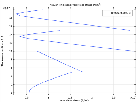
In the Settings window for 1D Plot Group, type von Mises Stress (Through-Thickness) in the Label text field.
3
Locate the Data section. From the Dataset list, choose Cut Point 3D 1.
Through Thickness 1
1
In the von Mises Stress (Through-Thickness) toolbar, click  More Plots and choose Through Thickness.
2
In the Settings window for Through Thickness, locate the x-Axis Data section.
3
In the Expression text field, type shell.mises.
4
Click to expand the Legends section. Select the Show legends check box.
5
In the von Mises Stress (Through-Thickness) toolbar, click  Plot.