PDF

Zone Electrophoresis
Introduction
Zone electrophoresis (ZE) is an electrophoretic separation technique, typically used for analyzing proteins, nucleic acids and biopolymers. During the process different species in a sample are transported in a continuous electrolyte buffer system, subject to a potential gradient. Due to differences in the mobilities, the species in the samples will eventually separate into different, well resolved, peaks.
This tutorial introduces the Electrophoretic Transport interface. A buffer system, consisting of a acetic acid and tris (tris(hydroxymethyl)aminomethane), is used to separate a sample consisting of pyridine and aniline into two well resolved peaks. The model is based on a review paper by Thormann and others(Ref. 1).
Model Definition
The model geometry is represented by an interval in 1D, representing the length (20 cm) of the separation column. The boundaries of the interval is assumed to be facing reservoirs containing large amounts of buffer electrolyte.
The transport of four different species is included: acetic acid, tris, aniline and pyridine. Acetic acid is defined as weak acid, whereas the other species are defined as weak bases. Each species is specified by a mobility and an acid constant (pKa). For the weak bases the pKa refers to the acid constant of the conjugate acid. Initial and boundary conditions are also specified for each species individually. The initial concentrations for acetic acid and tris are constant over the interval, whereas the sample concentration of aniline and pyridine is defined using a rectangular function with a width of 2.5% of the interval, located close to the leftmost boundary.
In addition to the species concentrations, the Electrophoretic Transport interface also solves for the pH and electrolyte potential distributions. A current density of 2500 A/m2 is applied at the end of the separation column.
The model is solved in a time-dependent solver, simulating the electrophoresis during 5 minutes.
Results and Discussion
Figures 1 to 4 show the distribution of pH, conductivity, tris and acetic acid at 0 and 4 minutes, respectively. Figure 1, showing the pH, features a rectangular imprint of the initial sample concentrations at 0 minutes, and a more complex distribution pattern at 4 minutes. Figure 2 shows a similar pattern, but with different relative peak heights.
Figure 1: pH distribution at 0 and 4 minutes.
Figure 2: Electrolyte conductivity at 0 and 4 minutes.
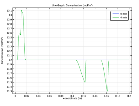
Figure 3 and Figure 4 show the concentration distribution of the buffer electrolyte species; tris and acetic acid. Note how the initial position of the sample at t=0 appears as “ghost” peaks in the buffer electrolyte after 4 minutes.
Figure 3: Concentration of tris at 0 and 4 minutes.
Figure 4: Concentration of acetic acid at 0 and 4 minutes.
Finally, Figure 5 and Figure 6 show the concentration of the pyridine and aniline sample at 1 and 3 minutes. The peaks are shaped as triangles, and the peak-to-peak distance increases as the samples move to the right in the separation column.
Figure 5: Sample concentrations at 1 min.
Figure 6: Sample concentrations at 3 min.
Reference
1. W Thormann, M Breadmore, J. Caslavska, and R. Mosher, “Dynamic computer simulations of electrophoresis: A versatile research and teaching tool,” Electrophoresis, vol. 31, pp. 726–754, 2010.
Application Library path: Chemical_Reaction_Engineering_Module/Electrokinetic_Effects/zone_electrophoresis
Modeling Instructions
From the File menu, choose New.
New
In the New window, click  Model Wizard.
Model Wizard
1
In the Model Wizard window, click  1D.
2
In the Select Physics tree, select Chemical Species Transport>Electrophoretic Transport (el).
3
Click Add.
4
Click  Study.
5
In the Select Study tree, select Preset Studies for Selected Physics Interfaces>Time Dependent with Initialization.
6
Global Definitions
Start by loading some model parameters from a text file.
Parameters 1
1
In the Model Builder window, under Global Definitions click Parameters 1.
2
In the Settings window for Parameters, locate the Parameters section.
3
Click  Load from File.
4
The parameter list now contains various parameters, such as L, T and mob_HAC etc. These will be used when defining the model.
Geometry 1
Draw the geometry of the model as an interval between 0 and the parameter L (=20 cm).
Interval 1 (i1)
1
In the Model Builder window, under Component 1 (comp1) right-click Geometry 1 and choose Interval.
2
In the Settings window for Interval, locate the Interval section.
3
4
Click  Build Selected.
Electrophoretic Transport (el)
Now start setting up the physics. A number of nodes have already been added by default.
Solvent 1
The Solvent node contains various settings relating to the aqueous solvent. Note that the temperature is set later in the Default Model Inputs node.
Insulation 1
An Insulation has also been created by default. It will later be overridden when you add the boundary conditions for the potential.
Initial Potential 1
If the model does not include potential dependent electrode reactions, the Initial Potential does not normally have to be set explicitly. Leave the setting as is.
Weak Base - tris
Now start adding various species nodes to the model. Begin with the weak base of the buffer electrolyte (tris).
1
In the Model Builder window, right-click Electrophoretic Transport (el) and choose Weak Base.
Each species added to the model adds its own equations, solving for a species concentration as the dependent variable. For a species with dissociation steps, the dependent concentration variable refers to the total concentration (the sum of all dissociated subspecies related to the species).
2
In the Settings window for Weak Base, type Weak Base - tris in the Label text field.
The Domain selection is set to All domains by default, so for this model there is no need to change this selection. However, the settings of the selection section can be used to specify that a species should only be present in certain parts of the geometry.
The Species name, which has to be unique, determines how the Electrophoretic Transport interface will name a number of variables, such as concentrations and fluxes.
3
Locate the Weak Base section. In the Species name text field, type tris.
The weak base node uses one dissociation reaction by default (Monoprotic), specified by one pKa value.
4
In the pKa text field, type pKa_tris.
5
Locate the Diffusion and Migration section. In the um text field, type mob_tris.
Initial Concentration 1
The boundary conditions and the initial values for a species are set by using child nodes.
The Initial Concentration node defines the concentration when the simulation starts.
1
In the Model Builder window, expand the Weak Base - tris node, then click Initial Concentration 1.
2
In the Settings window for Initial Concentration, locate the Initial Concentration section.
3
In the c text field, type tris_c0.
Weak Base - tris
The Concentration node defines the concentration at a boundary, in this case the inlet reservoir.
1
In the Model Builder window, click Weak Base - tris.
Concentration 1
1
In the Physics toolbar, click  Attributes and choose Concentration.
2
3
In the Settings window for Concentration, locate the Concentration section.
4
In the c0 text field, type tris_c0.
Weak Base - tris
The Outflow node defines a boundary with zero diffusive flux for the species. This is a suitable condition for at boundaries where the species is transported into a reservoir.
1
In the Model Builder window, click Weak Base - tris.
Outflow 1
1
In the Physics toolbar, click  Attributes and choose Outflow.
2
Weak Acid - HAC
Now proceed similarly to create the weak acid of the buffer electrolyte (HAC).
1
In the Physics toolbar, click  Domains and choose Weak Acid.
2
In the Settings window for Weak Acid, type Weak Acid - HAC in the Label text field.
3
Locate the Weak Acid section. In the Species name text field, type HAC.
4
In the pKa text field, type pKa_HAC.
5
Locate the Diffusion and Migration section. In the um text field, type mob_HAC.
Initial Concentration 1
1
In the Model Builder window, expand the Weak Acid - HAC node, then click Initial Concentration 1.
2
In the Settings window for Initial Concentration, locate the Initial Concentration section.
3
In the c text field, type HAC_c0.
Weak Acid - HAC
In the Model Builder window, click Weak Acid - HAC.
Concentration 1
1
In the Physics toolbar, click  Attributes and choose Concentration.
2
3
In the Settings window for Concentration, locate the Concentration section.
4
In the c0 text field, type HAC_c0.
Weak Acid - HAC
In the Model Builder window, click Weak Acid - HAC.
Outflow 1
1
In the Physics toolbar, click  Attributes and choose Outflow.
2
Weak Base - ani
Now start adding the samples (aniline and pyridine) that are to be separated during the zone electrophoresis. A quick way to do this can many times be to duplicate an existing node instead of creating it new from scratch.
1
In the Model Builder window, right-click Weak Base - tris and choose Duplicate.
2
In the Settings window for Weak Base, type Weak Base - ani in the Label text field.
3
Locate the Weak Base section. In the Species name text field, type ani.
4
In the pKa text field, type pKa_ani.
5
Locate the Diffusion and Migration section. In the um text field, type mob_ani.
Definitions
Since the initial sample concentrations are not uniform over the whole domain, we need to specify the initial values using functions.
Rectangle 1 (rect1)
1
In the Model Builder window, expand the Weak Base - ani node.
2
Right-click Component 1 (comp1)>Definitions and choose Functions>Rectangle.
The rectangle function creates a function between 0 and 1.
3
In the Settings window for Rectangle, click to expand the Smoothing section.
The transition between 0 and 1 is done smoothly instead of using a discrete step. This improves the numerics when solving the problem. Leave the smoothing settings as they are.
Sample function
There are a number of different function types available such as Gaussian Pulse, Interpolation, Step etc. Now add a second, Analytic, function to finalize the sample function. The function places the rectangle between 2.5% and 5% of the length of the geometry interval.
1
In the Home toolbar, click  Functions and choose Global>Analytic.
2
In the Settings window for Analytic, type Sample function in the Label text field.
3
In the Function name text field, type sample.
4
Locate the Definition section. In the Expression text field, type rect1((x-L*0.0375)/(L*0.025)).
5
Locate the Units section. In the Arguments text field, type m.
6
In the Function text field, type 1.
7
Locate the Plot Parameters section. In the table, enter the following settings:
8
Electrophoretic Transport (el)
Initial Concentration 1
Now use the sample function you just created to define the initial concentration distribution of the aniline species.
1
In the Model Builder window, under Component 1 (comp1)>Electrophoretic Transport (el)>Weak Base - ani click Initial Concentration 1.
2
In the Settings window for Initial Concentration, locate the Initial Concentration section.
3
In the c text field, type sample(x)*ani_c0.
Concentration 1
1
In the Model Builder window, click Concentration 1.
2
In the Settings window for Concentration, locate the Concentration section.
3
In the c0 text field, type 0.
Weak Base - ani
Proceed similarly to create the pyridine species.
Weak Base - pyr
1
In the Model Builder window, right-click Weak Base - ani and choose Duplicate.
2
In the Settings window for Weak Base, type Weak Base - pyr in the Label text field.
3
Locate the Weak Base section. In the Species name text field, type pyr.
4
In the pKa text field, type pKa_pyr.
5
Locate the Diffusion and Migration section. In the um text field, type mob_pyr.
Initial Concentration 1
1
In the Model Builder window, expand the Weak Base - pyr node, then click Initial Concentration 1.
2
In the Settings window for Initial Concentration, locate the Initial Concentration section.
3
In the c text field, type sample(x)*pyr_c0.
Potential 1
Finally, provide the boundary conditions for the electrolyte potential equation.
1
In the Physics toolbar, click  Boundaries and choose Potential.
A potential level always needs defined somewhere in the model, otherwise there will be no unique solution to the problem (which will render a solver error). In this case we will ground the left boundary.
2
Leave the default potential setting value (0[V]) as is.
Current Density 1
1
In the Physics toolbar, click  Boundaries and choose Current Density.
2
3
In the Settings window for Current Density, locate the Electrolyte Current Density section.
4
In the in,l text field, type -2500[A/m^2].
Note that we are specifying the value for the current density directly here, instead of using parameters (L etc.) as we did before. The brackets [ and ] are used to define the unit. (They may actually be omitted in this case since we are using the same units as the unit system of the model).
Global Definitions
Default Model Inputs
Set up the temperature value used in the entire model.
1
In the Model Builder window, under Global Definitions click Default Model Inputs.
2
In the Settings window for Default Model Inputs, locate the Browse Model Inputs section.
3
In the tree, select General>Temperature (K) - minput.T.
4
Find the Expression for remaining selection subsection. In the Temperature text field, type T.
Mesh 1
Solve the problem on a mesh consisting of 1000 elements.
1
In the Model Builder window, under Component 1 (comp1) click Mesh 1.
2
In the Settings window for Mesh, locate the Mesh Settings section.
3
From the Sequence type list, choose User-controlled mesh.
Distribution 1
1
In the Model Builder window, right-click Edge 1 and choose Distribution.
2
In the Settings window for Distribution, locate the Distribution section.
3
In the Number of elements text field, type 1000.
Once you have solved the model you can go back and increase the number of elements. This will increase the resolution of the concentration peaks in the solution, but will also increase the computation time.
4
Click  Build All.
For now, the finalized mesh should now look as follows:
Study 1
The problem is now ready for solving. Note that the Time dependent with Initialization study you added initially in the model wizard has created a study sequence consisting of one Current Distribution Initialization study step followed by one Time Dependent step. The initialization step is used to compute the initial potential and pH distribution before the time-dependent solver starts.
Step 2: Time Dependent
Set up the solver to solve between 0 and 5 minutes, storing the solution every 30 s.
1
In the Model Builder window, under Study 1 click Step 2: Time Dependent.
2
In the Settings window for Time Dependent, locate the Study Settings section.
3
From the Time unit list, choose min.
4
Click  Range.
5
In the Range dialog box, type 0.5 in the Step text field.
6
In the Stop text field, type 5.
7
Click Replace.
8
In the Home toolbar, click  Compute.
The model should now solve in about a minute or two.
Results
pH (el)
Plots for pH, conductivity, potential, and concentrations are created by default. To compare these to the plots in the Results and Discussion section, proceed as follows for each plot:
1
In the Settings window for 1D Plot Group, locate the Data section.
2
From the Time selection list, choose From list.
3
In the Times (min) list, choose 0 and 4.
4
In the pH (el) toolbar, click  Plot.
Sample concentrations
You can also create your own plots. Proceed as follows to create a plot that compares the aniline and pyridine concentrations in the same graph.
1
In the Model Builder window, right-click Molar Concentration - pyr (el) and choose Duplicate.
2
In the Settings window for 1D Plot Group, type Sample concentrations in the Label text field.
3
Locate the Data section. In the Times (min) list, select 1.
4
Click to expand the Title section. From the Title type list, choose Label.
Line Graph 1
1
In the Model Builder window, expand the Sample concentrations node, then click Line Graph 1.
2
In the Settings window for Line Graph, locate the y-Axis Data section.
3
In the Unit field, type mM.
4
Locate the x-Axis Data section. From the Unit list, choose cm.
5
Click to expand the Legends section. From the Legends list, choose Manual.
6
Line Graph 2
1
Right-click Results>Sample concentrations>Line Graph 1 and choose Duplicate.
2
In the Settings window for Line Graph, click Replace Expression in the upper-right corner of the y-Axis Data section. From the menu, choose Component 1 (comp1)>Electrophoretic Transport>Weak Base - ani>el.c_ani - Concentration - mol/m³.
3
Locate the Legends section. In the table, enter the following settings:
Sample concentrations
You can now compare the concentrations at 1 and 3 min as follows:
1
In the Model Builder window, click Sample concentrations.
2
In the Sample concentrations toolbar, click  Plot.
3
In the Settings window for 1D Plot Group, locate the Data section.
4
In the Times (min) list, select 3.
5
In the Sample concentrations toolbar, click  Plot.
Animation 1
You can also create an animation of the plot you just created, for all times stored in the solution.
1
In the Results toolbar, click  Animation and choose Player.
2
In the Settings window for Animation, locate the Scene section.
3
From the Subject list, choose Sample concentrations.
4
Locate the Frames section. From the Frame selection list, choose All.
5
Locate the Playing section. In the Display each frame for text field, type 0.5.
6
Right-click Animation 1 and choose Play.
Increasing the number of frames in the animation can be achieved by decreasing the incremental step of the range() operator, for example range(0,0.1,5) under Times in the Time Dependent node, and re-solving.