PDF

Steam Reformer
Introduction
This example illustrates the modeling of a steam reformer, serving a stationary fuel cell unit with hydrogen. The tightly coupled system of mass, energy, and momentum equations used to describe the system, is readily set up using the predefined physics interfaces of the Chemical Reaction Engineering Module.
Model Definition
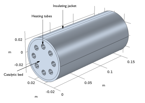
In fuel cell power generators, a steam reformer unit typically produces the hydrogen needed for the cell stack. Figure 1 shows the geometry of such a system. The reformation chemistry occurs in a porous catalytic bed where energy is supplied through heating tubes to drive the endothermic process. The reactor is enclosed in an insulating jacket.
Figure 1: Geometry of the steam reformer unit.
In this example, propane and steam are mixed in stoichiometric amounts and enter through the inlet of the reactor. For heating purposes, hot gases from a burner are passed in the opposite direction, through a number of tubes perforating the reactor bed.
Figure 2: Making use of symmetry, the modeling domain is reduced to a quarter of the full geometry.
In the reformer, water and propane react to form hydrogen and carbon dioxide:
An overall kinetic model has been established from experiments (Ref. 1), where the reaction rate (SI unit: mol/(m3·s)) has been found to be first order in the propane concentration:
(1)
The rate constant follows Arrhenius equation, with the temperature dependence:
where the frequency factor A is 7·105 s-1 and the activation energy Ea is 83.14 kJ/mol.
Fluid Flow — reformer Bed
The flow of gaseous species through the reformer bed is described by Darcy’s law:
Here, ρ denotes the gas density (SI unit: kg/m3), η the viscosity (SI unit: Pa·s), κ the permeability of the porous medium (SI unit: m2), and psr is the pressure in the reformer bed (SI unit: Pa). The Darcy’s law equation is, in this example, solved with the Darcy’s law interface.
The inlet and outlet boundary conditions describe a 50 Pa pressure drop across the bed. All other boundaries are impervious, corresponding to the condition:
Energy Transport — reformer Bed
A one-equation approach is used to describe the average temperature distribution in the porous bed:
The effective thermal conductivity of the bed, keff (SI unit: W/(m·K)), is given by:
In the above equations, the indices “f” and “pm” denote fluid and porous matrix, respectively, and ε is the volume fraction of the fluid phase. The effective volumetric heat capacity of the bed is given by:
Furthermore, Tsr is the temperature (SI unit: K), Q represents a heat source (SI unit: W/m3), and u the fluid velocity (SI unit: m/s). The equation is modeled using the Heat Transfer in Porous Media interface.
Assuming that the porous medium is homogeneous and isotropic, the steady-state equation becomes
(2)
The heat source due to reaction is
where, r is given by Equation 1. The steam reformation of propane is endothermic, with an enthalpy of reaction of ΔHr = 410 kJ/mol.
Equation 2 also accounts for the conductive heat transfer in the insulating jacket. As no reactions occur in this domain, the description reduces to:
where ki is the thermal conductivity (W/(m·K)) of the insulating material.
The temperature of the gas is 700 K at the inlet. At the outlet, it is assumed that convective heat transport is dominant:
The heat exchange between the bed and the tubes is described by:
(3)
where hht is the heat transfer coefficient (SI unit: W/(m2·K)) and T is the temperature (K) of the heating tubes. A similar expression describes the heat flux from the insulating jacket to the surroundings:
where hj is the heat transfer coefficient of the jacket (SI unit: W/(m2·K)) and Tamb is the ambient temperature (K).
Mass Transport — reformer Bed
The Transport of Concentrated Species interface gives the equations for the mass transport. The mass-balance equations for the model are the Maxwell-Stefan diffusion and convection equations at steady state:
In the equations above, ρ denotes the density (kg/m3), ωi is the mass fraction of species i, xk is the molar fraction of species k, is the ik component of the effective multicomponent Fick diffusivity (m2/s). denotes the effective generalized thermal diffusion coefficient (kg/(m·s)), T is the temperature (K), and Ri the reaction rate (kg/(m3·s)). The mass-balances are set up and solved with the Transport of Concentrated Species interface. The effective parameters accounts for the impact of porosity on the diffusivity, this model uses the Millington and Quirk model:
The inlet weight fraction of propane is 0.28. At the outlet, the convective flux condition is used:
All other boundaries use the insulating or symmetry condition.
Fluid Flow — heating Tubes
The flow of heating gas in the tubes is described by the weakly compressible Navier-Stokes equations at steady-state:
where ρ denotes density (SI unit: kg/m3), u represents the velocity (SI unit: m/s), μ denotes dynamic viscosity (SI unit: kg/(m· s)), and p equals the pressure in the tubes (SI unit: Pa).
The boundary conditions are
At the outlet, viscous stresses are ignored and the pressure is set to 1 atmosphere.
The Laminar Flow interface sets up and solves the Navier-Stokes equations and is here used to model the gas flow in the tubes. Since the flow is nonisothermal, the Heat Transfer in Fluids interface is also used. These interfaces are coupled through the Nonisothermal Flow multiphysics coupling feature.
Energy Transport — heating Tubes
The energy transport in heating tubes is described by:
where kht is the thermal conductivity (SI unit: W/(m·K)) of the heating gas. The temperature of the gas is 900 K at the inlet. Also this energy transport is modeled with the Heat Transfer in Fluids interface.
At the outlet, it is assumed that convective heat transport is dominant:
The heat exchange between the bed and tubes is given by:
This is the same heat flux as given by Equation 3, but with reversed sign.
Results and Discussion
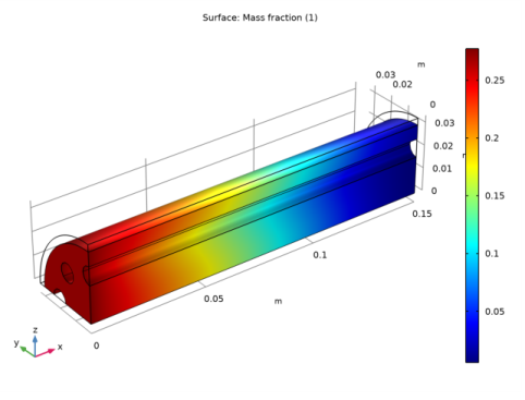
Figure 3 shows the weight fraction of propane in the reformer bed. The inlet weight fraction is 0.28 while the fraction at the outlet is close to zero.
Figure 3: Weight fraction distribution of propane in the reformer bed.
A cross section plot through the center of the reformer reveals a concentration distribution in the bed. As the local reactivity is mainly controlled by the temperature, results indicate the heat supplied by the tubes is sufficient to efficiently make use of the entire catalytic bed.
Figure 4: Weight fraction distribution of propane in a cross section through the middle of the reformer bed.
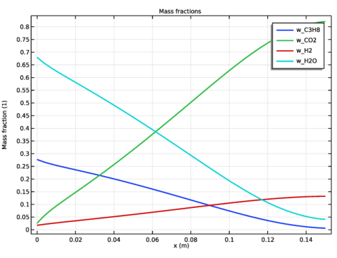
Figure 5 shows the weight fractions of all reacting species in the bed, evaluated along the reactor centerline. The plot shows that the entire bed length is active in converting propane.
Figure 5: Weight fraction of reacting species as function of reactor position, plotted along the reactor centerline.
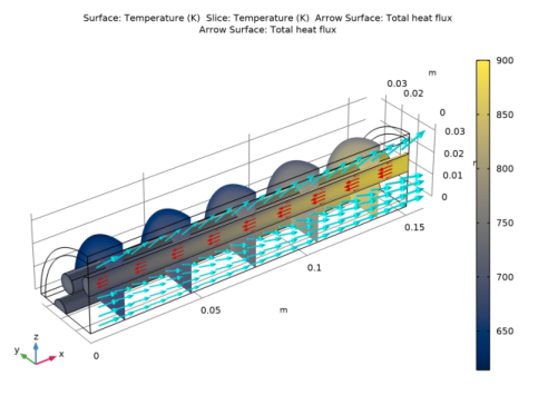
The energy exchange between the heating tubes and reformer bed is clearly illustrated in Figure 6. The gas of the heating tubes enters at 900 K and exits at approximately 716 K. The gas temperature in the reformer bed is 700 K at the inlet, goes through a minimum, and finally exits with an average temperature of 843 K.
Figure 6: Temperature distributions in the reformer system, including the reformer bed, heating tubes and insulating wall.
A line plot through the center of the reactor shows how the temperature initially decreases due to the endothermic reformation reactions. When the reaction rate is reduced as a function of lower temperature and propane content, the energy supplied by the heating tubes dictates the temperature evolution.
Figure 7: Bed temperature as a function of position, plotted along the reactor centerline.
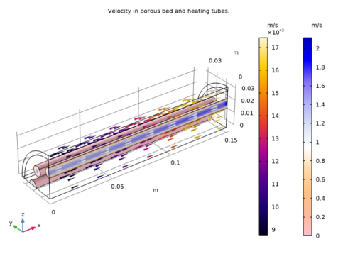
Figure 8 shows the velocity fields of both the heating gas in the tubes and the reacting gas in the bed. The flow in the heating tubes is laminar and the parabolic velocity distribution is clearly seen. The gas velocity in the porous bed increases significantly through the reactor, and, at the outlet, the gas velocity is approximately than twice that at the inlet.
Figure 8: Velocity fields of the heating tubes and the reformer bed.
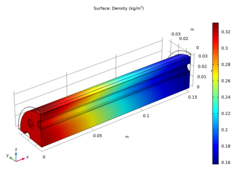
The increased velocity is mainly due to gas expansion caused by chemical reaction and, to a lesser extent, by temperature increase. Figure 9 illustrates the associated density variations in the reformer bed, accounting for both composition and temperature effects.
Figure 9: Overall gas density in the reformer bed.
In summary, this example illustrates the simulation of a reactor described by fully coupled mass, energy and flow equations.
Reference
1. P.Gateau, Design of Reactors and Heat Exchange Systems to Optimize a Fuel Cell Reformer, Proceedings of the COMSOL User’s Conference Grenoble, 2007.
Application Library path: Chemical_Reaction_Engineering_Module/Reactors_with_Porous_Catalysts/steam_reformer
Modeling Instructions
From the File menu, choose New.
New
In the New window, click  Blank Model.
Global Definitions
In the Model Builder window, right-click Global Definitions and choose Thermodynamics>Thermodynamic System.
Select System
1
Go to the Select System window.
2
Click Next in the window toolbar.
Select Species
1
Go to the Select Species window.
2
In the Species list, select propane (74-98-6, C3H8).
3
Click  Add Selected.
4
In the Species list, select water (7732-18-5, H2O).
5
Click  Add Selected.
6
In the Species list, select hydrogen (1333-74-0, H2).
7
Click  Add Selected.
8
In the Species list, select carbon dioxide (124-38-9, CO2).
9
Click  Add Selected.
10
Click Next in the window toolbar.
Select Thermodynamic Model
1
Go to the Select Thermodynamic Model window.
2
Click Finish in the window toolbar.
Global Definitions
Gas System 1 (pp1)
In the Model Builder window, under Global Definitions>Thermodynamics right-click Gas System 1 (pp1) and choose Generate Chemistry.
Select Species
1
Go to the Select Species window.
2
Click  Add All.
3
Click Next in the window toolbar.
Chemistry Settings
1
Go to the Chemistry Settings window.
2
From the Mass transfer list, choose Concentrated species.
3
Click Finish in the window toolbar.
Geometry 1
Now create the geometry. To simplify this step, insert a prepared geometry sequence:
1
In the Model Builder window, under Component 1 (comp1) click Geometry 1.
2
In the Geometry toolbar, point to Import/Export and choose Insert Sequence.
3
4
Click Build All in the Geometry toolbar.
Definitions
Catalytic Bed
1
In the Definitions toolbar, click  Explicit.
2
In the Settings window for Explicit, type Catalytic Bed in the Label text field.
3
Remaining explicit definitions
Analogous to the explicit definition for the Catalytic Bed, proceed to create the following explicit definitions:
Also create a union selection containing all inlet and outlet boundaries. This will be used to refine the mesh in these areas.
Inlets and Outlets
1
In the Definitions toolbar, click  Union.
2
In the Settings window for Union, type Inlets and Outlets in the Label text field.
3
Locate the Geometric Entity Level section. From the Level list, choose Boundary.
4
Locate the Input Entities section. Under Selections to add, click  Add.
5
In the Add dialog box, in the Selections to add list, choose Bed Inlet, Bed Outlet, Tubes Inlet, and Tubes Outlet.
6
Integration 1 (intop1)
1
In the Definitions toolbar, click  Nonlocal Couplings and choose Integration.
2
In the Settings window for Integration, locate the Source Selection section.
3
From the Geometric entity level list, choose Boundary.
4
Global Definitions
A set of parameters useful when building the model are available in a text file.
Parameters 1
1
In the Model Builder window, under Global Definitions click Parameters 1.
2
In the Settings window for Parameters, locate the Parameters section.
3
Click  Load from File.
4
Add Physics
1
In the Home toolbar, click  Add Physics to open the Add Physics window.
2
Go to the Add Physics window.
3
In the tree, select Chemical Species Transport>Transport of Concentrated Species (tcs).
4
Click Add to Component 1 in the window toolbar.
Transport of Concentrated Species (tcs)
1
In the Settings window for Transport of Concentrated Species, locate the Transport Mechanisms section.
2
Select the Mass transfer in porous media check box.
3
Click to expand the Dependent Variables section. In the Number of species text field, type 4.
4
In the Mass fractions table, enter the following settings:
Add Physics
1
Go to the Add Physics window.
2
In the tree, select Fluid Flow>Porous Media and Subsurface Flow>Darcy’s Law (dl).
3
Click Add to Component 1 in the window toolbar.
Darcy’s Law (dl)
1
In the Settings window for Darcy’s Law, locate the Physical Model section.
2
In the pref text field, type p_ref.
3
Click to expand the Dependent Variables section. In the Pressure text field, type p_sr.
Add Physics
1
Go to the Add Physics window.
2
In the tree, select Heat Transfer>Heat Transfer in Porous Media (ht).
3
Click Add to Component 1 in the window toolbar.
Heat Transfer in Porous Media (ht)
1
In the Settings window for Heat Transfer in Porous Media, click to expand the Dependent Variables section.
2
In the Temperature text field, type T_sr.
Add Physics
1
Go to the Add Physics window.
2
In the tree, select Fluid Flow>Nonisothermal Flow>Laminar Flow.
3
Click Add to Component 1 in the window toolbar.
4
In the Home toolbar, click  Add Physics to close the Add Physics window.
Laminar Flow (spf)
1
In the Settings window for Laminar Flow, locate the Physical Model section.
2
In the pref text field, type p_ref.
3
Click to expand the Dependent Variables section. In the Pressure text field, type p_tubes.
Heat Transfer in Fluids 2 (ht2)
1
In the Model Builder window, under Component 1 (comp1) click Heat Transfer in Fluids 2 (ht2).
2
In the Settings window for Heat Transfer in Fluids, click to expand the Dependent Variables section.
3
In the Temperature text field, type T_tubes.
Chemistry (chem)
1
In the Model Builder window, under Component 1 (comp1) click Chemistry (chem).
2
In the Settings window for Chemistry, locate the Species Matching section.
3
Find the Bulk species subsection. In the table, enter the following settings:
4
Click to expand the Calculate Transport Properties section. Click to collapse the Calculate Transport Properties section.
Reaction 1
1
In the Physics toolbar, click  Domains and choose Reaction.
2
In the Settings window for Reaction, locate the Reaction Formula section.
3
In the Formula text field, type C3H8 + H2O => H2 + CO2.
4
Click Balance in the upper-right corner of the Reaction Formula section.
5
Locate the Reaction Rate section. From the list, choose User defined.
6
In the rj text field, type chem.kf_1*chem.c_C3H8.
7
Find the Volumetric overall reaction order subsection. In the Forward text field, type 1.
8
Locate the Rate Constants section. Select the Use Arrhenius expressions check box.
9
In the Af text field, type A.
10
In the Ef text field, type Ea.
Transport of Concentrated Species in Bed
1
In the Model Builder window, under Component 1 (comp1) click Transport of Concentrated Species (tcs).
2
In the Settings window for Transport of Concentrated Species, type Transport of Concentrated Species in Bed in the Label text field.
3
Locate the Domain Selection section. From the Selection list, choose Catalytic Bed.
4
Locate the Transport Mechanisms section. From the Diffusion model list, choose Maxwell-Stefan.
Initial Values 1
1
In the Model Builder window, under Component 1 (comp1)>Transport of Concentrated Species in Bed (tcs) click Initial Values 1.
2
In the Settings window for Initial Values, locate the Initial Values section.
3
In the ω0,wC3H8 text field, type w_C3H8_in.
4
In the ω0,wH2 text field, type w_H2_in.
5
In the ω0,wCO2 text field, type w_CO2_in.
Porous Media Transport Properties 1
1
In the Physics toolbar, click  Domains and choose Porous Media Transport Properties.
2
In the Settings window for Porous Media Transport Properties, locate the Domain Selection section.
3
From the Selection list, choose Catalytic Bed.
4
Locate the Matrix Properties section. In the εp text field, type porosity.
5
Locate the Density section. From the MwH2O list, choose Molar mass (chem/H2O).
6
From the MwC3H8 list, choose Molar mass (chem/C3H8).
7
From the MwH2 list, choose Molar mass (chem/H2).
8
From the MwCO2 list, choose Molar mass (chem/CO2).
9
Locate the Convection section. From the u list, choose Darcy’s velocity field (dl).
10
Locate the Diffusion section. In the table, enter the following settings:
Reaction Sources 1
1
In the Physics toolbar, click  Domains and choose Reaction Sources.
2
In the Settings window for Reaction Sources, locate the Domain Selection section.
3
From the Selection list, choose Catalytic Bed.
4
Locate the Reactions section. From the RwC3H8 list, choose Reaction rate for species C3H8 (chem).
5
From the RwH2 list, choose Reaction rate for species H2 (chem).
6
From the RwCO2 list, choose Reaction rate for species CO2 (chem).
7
Locate the Reacting Volume section. From the Reacting volume list, choose Pore volume.
Inflow 1
In the Physics toolbar, click  Boundaries and choose Inflow.
Definitions
Variables 1
1
In the Home toolbar, click  Variables and choose Local Variables.
2
In the Settings window for Variables, locate the Variables section.
3
Transport of Concentrated Species in Bed (tcs)
Inflow 1
1
In the Model Builder window, under Component 1 (comp1)>Transport of Concentrated Species in Bed (tcs) click Inflow 1.
2
In the Settings window for Inflow, locate the Boundary Selection section.
3
From the Selection list, choose Bed Inlet.
4
Locate the Inflow section. From the Mixture specification list, choose Mass flow rates.
5
In the Jin,wC3H8 text field, type J_in_C3H8.
6
In the Jin,wH2 text field, type J_in_H2.
7
In the Jin,wCO2 text field, type J_in_CO2.
Outflow 1
1
In the Physics toolbar, click  Boundaries and choose Outflow.
2
In the Settings window for Outflow, locate the Boundary Selection section.
3
From the Selection list, choose Bed Outlet.
Darcy’s Law in Bed
1
In the Model Builder window, under Component 1 (comp1) click Darcy’s Law (dl).
2
In the Settings window for Darcy’s Law, type Darcy's Law in Bed in the Label text field.
3
Locate the Domain Selection section. Click  Remove from Selection.
4
From the Selection list, choose Catalytic Bed.
Fluid and Matrix Properties 1
1
In the Model Builder window, under Component 1 (comp1)>Darcy’s Law in Bed (dl) click Fluid and Matrix Properties 1.
2
In the Settings window for Fluid and Matrix Properties, locate the Fluid Properties section.
3
From the ρ list, choose Density (tcs).
4
From the μ list, choose Dynamic viscosity (chem).
5
Locate the Matrix Properties section. From the εp list, choose User defined. In the associated text field, type porosity.
6
From the κ list, choose User defined. In the associated text field, type kappa_pm.
Inlet 1
1
In the Physics toolbar, click  Boundaries and choose Inlet.
2
In the Settings window for Inlet, locate the Boundary Condition section.
3
4
Locate the Pressure section. In the p0 text field, type p_in_sr.
5
Locate the Boundary Selection section. From the Selection list, choose Bed Inlet.
Outlet 1
1
In the Physics toolbar, click  Boundaries and choose Outlet.
2
In the Settings window for Outlet, locate the Boundary Selection section.
3
From the Selection list, choose Bed Outlet.
4
Locate the Boundary Condition section. From the list, choose Pressure.
Symmetry 1
1
In the Physics toolbar, click  Boundaries and choose Symmetry.
2
In the Settings window for Symmetry, locate the Boundary Selection section.
3
From the Selection list, choose Bed Symmetry.
Heat Transfer in Porous Media in Bed
1
In the Model Builder window, under Component 1 (comp1) click Heat Transfer in Porous Media (ht).
2
In the Settings window for Heat Transfer in Porous Media, type Heat Transfer in Porous Media in Bed in the Label text field.
3
Locate the Domain Selection section. From the Selection list, choose Catalytic Bed.
4
Fluid 1
1
In the Model Builder window, expand the Component 1 (comp1)>Heat Transfer in Porous Media in Bed (ht)>Porous Medium 1 node, then click Fluid 1.
2
In the Settings window for Fluid, locate the Heat Convection section.
3
From the u list, choose Darcy’s velocity field (dl).
4
Locate the Heat Conduction, Fluid section. From the kf list, choose Thermal conductivity (chem).
5
Locate the Thermodynamics, Fluid section. From the ρf list, choose Density (tcs).
6
From the Cp,f list, choose Heat capacity at constant pressure (chem).
7
From the γ list, choose Ratio of specific heats (chem).
Porous Matrix 1
1
In the Model Builder window, click Porous Matrix 1.
2
In the Settings window for Porous Matrix, locate the Matrix Properties section.
3
From the εp list, choose User defined. In the associated text field, type porosity.
4
From the Define list, choose Solid phase properties.
5
Locate the Heat Conduction, Porous Matrix section. From the ks list, choose User defined. In the associated text field, type k_pm.
6
Locate the Thermodynamics, Porous Matrix section. From the ρs list, choose User defined. In the associated text field, type dens_pm.
7
From the Cp,s list, choose User defined. In the associated text field, type Cp_pm.
Initial Values 1
1
In the Model Builder window, click Initial Values 1.
2
In the Settings window for Initial Values, locate the Initial Values section.
3
In the Tsr text field, type T_in_sr.
Solid 1
1
In the Physics toolbar, click  Domains and choose Solid.
2
In the Settings window for Solid, locate the Domain Selection section.
3
From the Selection list, choose Jacket.
4
Locate the Heat Conduction, Solid section. From the k list, choose User defined. In the associated text field, type k_foam.
5
Locate the Thermodynamics, Solid section. From the ρ list, choose User defined. In the associated text field, type dens_foam.
6
From the Cp list, choose User defined. In the associated text field, type Cp_foam.
Temperature 1
1
In the Physics toolbar, click  Boundaries and choose Temperature.
2
In the Settings window for Temperature, locate the Boundary Selection section.
3
From the Selection list, choose Bed Inlet.
4
Locate the Temperature section. In the T0 text field, type T_in_sr.
Outflow 1
1
In the Physics toolbar, click  Boundaries and choose Outflow.
2
In the Settings window for Outflow, locate the Boundary Selection section.
3
From the Selection list, choose Bed Outlet.
Heat Flux 1
1
In the Physics toolbar, click  Boundaries and choose Heat Flux.
2
In the Settings window for Heat Flux, locate the Boundary Selection section.
3
From the Selection list, choose Tubes/Bed.
4
Locate the Heat Flux section. Click the Convective heat flux button.
5
In the h text field, type h_tubes.
6
In the Text text field, type T_tubes.
Heat Flux 2
1
In the Physics toolbar, click  Boundaries and choose Heat Flux.
2
In the Settings window for Heat Flux, locate the Boundary Selection section.
3
From the Selection list, choose Jacket/Ambient.
4
Locate the Heat Flux section. Click the Convective heat flux button.
5
In the h text field, type h_j.
6
In the Text text field, type T_amb.
Heat Source 1
1
In the Physics toolbar, click  Domains and choose Heat Source.
2
In the Settings window for Heat Source, locate the Heat Source section.
3
In the Q0 text field, type porosity*chem.Qtot.
4
Locate the Domain Selection section. From the Selection list, choose Catalytic Bed.
Add Material
1
In the Home toolbar, click  Add Material to open the Add Material window.
2
Go to the Add Material window.
3
In the Search text field, type air.
4
Click Search.
5
In the tree, select Liquids and Gases>Gases>Air.
6
Click  Add to Component 1 (comp1).
7
In the Home toolbar, click  Add Material to close the Add Material window.
Materials
Air (mat1)
1
In the Settings window for Material, locate the Geometric Entity Selection section.
2
From the Selection list, choose Heating Tubes.
Laminar Flow in Heating Tubes
1
In the Model Builder window, under Component 1 (comp1) click Laminar Flow (spf).
2
In the Settings window for Laminar Flow, type Laminar Flow in Heating Tubes in the Label text field.
3
Locate the Domain Selection section. From the Selection list, choose Heating Tubes.
Inlet 1
1
In the Physics toolbar, click  Boundaries and choose Inlet.
2
In the Settings window for Inlet, locate the Boundary Selection section.
3
From the Selection list, choose Tubes Inlet.
4
Locate the Boundary Condition section. From the list, choose Fully developed flow.
5
Locate the Fully Developed Flow section. In the Uav text field, type u_in_tubes.
Outlet 1
1
In the Physics toolbar, click  Boundaries and choose Outlet.
2
In the Settings window for Outlet, locate the Boundary Selection section.
3
From the Selection list, choose Tubes Outlet.
4
Locate the Pressure Conditions section. Select the Normal flow check box.
Symmetry 1
1
In the Physics toolbar, click  Boundaries and choose Symmetry.
2
In the Settings window for Symmetry, locate the Boundary Selection section.
3
From the Selection list, choose Tubes Symmetry.
Heat Transfer in Heating Tubes
1
In the Model Builder window, under Component 1 (comp1) click Heat Transfer in Fluids 2 (ht2).
2
In the Settings window for Heat Transfer in Fluids, type Heat Transfer in Heating Tubes in the Label text field.
3
Locate the Domain Selection section. From the Selection list, choose Heating Tubes.
Initial Values 1
1
In the Model Builder window, under Component 1 (comp1)>Heat Transfer in Heating Tubes (ht2) click Initial Values 1.
2
In the Settings window for Initial Values, locate the Initial Values section.
3
In the Ttubes text field, type T_in_tubes.
Temperature at Inlet
1
In the Physics toolbar, click  Boundaries and choose Temperature.
2
In the Settings window for Temperature, type Temperature at Inlet in the Label text field.
3
Locate the Boundary Selection section. From the Selection list, choose Tubes Inlet.
4
Locate the Temperature section. In the T0 text field, type T_in_tubes.
Outflow 1
1
In the Physics toolbar, click  Boundaries and choose Outflow.
2
In the Settings window for Outflow, locate the Boundary Selection section.
3
From the Selection list, choose Tubes Outlet.
Heat Flux to bed
1
In the Physics toolbar, click  Boundaries and choose Heat Flux.
2
In the Settings window for Heat Flux, type Heat Flux to bed in the Label text field.
3
Locate the Boundary Selection section. From the Selection list, choose Tubes/Bed.
4
Locate the Heat Flux section. Click the Convective heat flux button.
5
In the h text field, type h_tubes.
6
In the Text text field, type T_sr.
Mesh 1
Free Triangular 1
1
In the Mesh toolbar, click  Boundary and choose Free Triangular.
2
Free Quad 1
1
In the Mesh toolbar, click  Boundary and choose Free Quad.
2
In the Settings window for Free Quad, locate the Boundary Selection section.
3
From the Selection list, choose Bed Inlet.
Boundary Layers 1
1
In the Mesh toolbar, click  Boundary Layers.
2
In the Settings window for Boundary Layers, locate the Geometric Entity Selection section.
3
From the Geometric entity level list, choose Boundary.
4
Boundary Layer Properties
1
In the Model Builder window, click Boundary Layer Properties.
2
3
In the Settings window for Boundary Layer Properties, locate the Boundary Layer Properties section.
4
In the Number of boundary layers text field, type 3.
5
From the Thickness of first layer list, choose Manual.
6
In the Thickness text field, type 3e-4.
Swept 1
In the Mesh toolbar, click  Swept.
Distribution 1
1
Right-click Swept 1 and choose Distribution.
2
In the Settings window for Distribution, locate the Distribution section.
3
In the Number of elements text field, type 50.
Size
1
In the Model Builder window, click Size.
2
In the Settings window for Size, locate the Element Size section.
3
Click the Custom button.
4
Locate the Element Size Parameters section. In the Maximum element size text field, type 2e-3.
5
In the Minimum element size text field, type 1e-3.
Boundary Layers 2
1
In the Mesh toolbar, click  Boundary Layers.
2
In the Settings window for Boundary Layers, click to expand the Transition section.
3
Clear the Smooth transition to interior mesh check box.
Boundary Layer Properties
1
In the Model Builder window, click Boundary Layer Properties.
2
In the Settings window for Boundary Layer Properties, locate the Geometric Entity Selection section.
3
From the Geometric entity level list, choose Boundary.
4
From the Selection list, choose Inlets and Outlets.
5
Locate the Boundary Layer Properties section. In the Number of boundary layers text field, type 6.
6
From the Thickness of first layer list, choose Manual.
7
In the Thickness text field, type 0.0003.
8
In the Model Builder window, right-click Mesh 1 and choose Build All.
Add Study
1
In the Home toolbar, click  Add Study to open the Add Study window.
2
Go to the Add Study window.
3
Find the Studies subsection. In the Select Study tree, select General Studies>Stationary.
4
Click  Add Study.
Study 1
Solution 1 (sol1)
In the Study toolbar, click  Show Default Solver.
Stationary 2
In the Study toolbar, click  Study Steps and choose Stationary>Stationary.
Step 1: Stationary
1
In the Model Builder window, click Step 1: Stationary.
2
In the Settings window for Stationary, locate the Physics and Variables Selection section.
3
In the table, clear the Solve for check boxes for Transport of Concentrated Species in Bed (tcs), Heat Transfer in Porous Media in Bed (ht), and Heat Transfer in Heating Tubes (ht2).
Solution 1 (sol1)
1
In the Study toolbar, click  Show Default Solver.
2
In the Model Builder window, expand the Solution 1 (sol1) node.
3
In the Model Builder window, expand the Study 1>Solver Configurations>Solution 1 (sol1)>Stationary Solver 2 node.
4
Right-click Stationary Solver 2 and choose Fully Coupled.
5
In the Settings window for Stationary Solver, locate the General section.
6
In the Relative tolerance text field, type 0.1.
7
In the Study toolbar, click  Compute.
Results
In the first part of the results processing, create the default plots giving Figure 3, Figure 4 and Figure 8.
Velocity (dl)
1
In the Model Builder window, expand the Results>Velocity (dl) node, then click Velocity (dl).
2
In the Settings window for 3D Plot Group, click to expand the Title section.
Streamline 1
1
In the Model Builder window, click Streamline 1.
2
In the Settings window for Streamline, click to expand the Quality section.
Color Expression 1
1
In the Model Builder window, expand the Streamline 1 node, then click Color Expression 1.
2
In the Settings window for Color Expression, locate the Coloring and Style section.
3
From the Color table list, choose HeatCamera.
Streamline 1
1
In the Model Builder window, click Streamline 1.
2
In the Settings window for Streamline, locate the Streamline Positioning section.
3
In the Points text field, type 6.
Volume 1
1
In the Model Builder window, right-click Velocity (dl) and choose Volume.
2
In the Settings window for Volume, click Replace Expression in the upper-right corner of the Expression section. From the menu, choose Component 1 (comp1)>Laminar Flow in Heating Tubes>Velocity and pressure>spf.U - Velocity magnitude - m/s.
Selection 1
1
Right-click Volume 1 and choose Selection.
2
In the Settings window for Selection, locate the Selection section.
3
From the Selection list, choose Heating Tubes.
Streamline 1
1
In the Model Builder window, click Streamline 1.
2
In the Settings window for Streamline, locate the Streamline Positioning section.
3
In the Points text field, type 20.
4
From the Positioning list, choose Uniform density.
5
In the Separating distance text field, type .05.
Volume 1
1
In the Model Builder window, click Volume 1.
2
In the Settings window for Volume, locate the Coloring and Style section.
3
From the Color table list, choose Twilight.
Streamline 1
1
In the Model Builder window, click Streamline 1.
2
In the Settings window for Streamline, locate the Coloring and Style section.
3
Find the Point style subsection. From the Arrow type list, choose Cone.
4
Find the Line style subsection. From the Type list, choose None.
Arrow Surface 1
1
In the Model Builder window, right-click Velocity (dl) and choose Arrow Surface.
2
In the Settings window for Arrow Surface, click Replace Expression in the upper-right corner of the Expression section. From the menu, choose Component 1 (comp1)>Laminar Flow in Heating Tubes>Velocity and pressure>u,v,w - Velocity field.
Selection 1
1
Right-click Arrow Surface 1 and choose Selection.
2
In the Settings window for Selection, locate the Selection section.
3
From the Selection list, choose Tubes Symmetry.
Arrow Surface 1
1
In the Model Builder window, click Arrow Surface 1.
2
In the Settings window for Arrow Surface, locate the Coloring and Style section.
3
From the Arrow type list, choose Cone.
4
Locate the Arrow Positioning section. In the Number of arrows text field, type 40.
5
From the Placement list, choose Uniform anisotropic.
6
In the x weight text field, type .4.
7
In the z weight text field, type 4.
8
Locate the Coloring and Style section. From the Color list, choose White.
Velocity
1
In the Model Builder window, under Results click Velocity (dl).
2
In the Settings window for 3D Plot Group, type Velocity in the Label text field.
3
Locate the Title section. From the Title type list, choose Manual.
4
In the Title text area, type Velocity in porous bed and heating tubes..
5
Locate the Color Legend section. Select the Show units check box.
6
In the Velocity toolbar, click  Plot.
This is Figure 8.
The 3D plot group showing the velocity field in the tubes can be deleted, since this was visualized in the previous plot.
Velocity (spf)
In the Model Builder window, right-click Velocity (spf) and choose Delete.
Mass fraction propane midreactor
1
In the Home toolbar, click  Add Plot Group and choose 3D Plot Group.
2
In the Settings window for 3D Plot Group, type Mass fraction propane midreactor in the Label text field.
3
Locate the Plot Settings section. Clear the Plot dataset edges check box.
Slice 1
1
Right-click Mass fraction propane midreactor and choose Slice.
2
In the Settings window for Slice, locate the Expression section.
3
In the Expression text field, type w_C3H8.
4
Locate the Plane Data section. In the Planes text field, type 1.
5
Locate the Coloring and Style section. From the Color table list, choose JupiterAuroraBorealis.
6
Locate the Plane Data section. In the Planes text field, type 3.
7
In the Mass fraction propane midreactor toolbar, click  Plot.
8
In the Planes text field, type 1.
9
In the Mass fraction propane midreactor toolbar, click  Plot.
Surface 1
In the Model Builder window, right-click Mass fraction propane midreactor and choose Surface.
Selection 1
1
In the Model Builder window, right-click Surface 1 and choose Selection.
2
3
In the Settings window for Selection, locate the Selection section.
4
Click  Remove from Selection.
5
6
Click  Remove from Selection.
7
8
Surface 1
1
In the Model Builder window, click Surface 1.
2
In the Settings window for Surface, locate the Expression section.
3
In the Expression text field, type 1.
4
Locate the Coloring and Style section. From the Coloring list, choose Uniform.
5
From the Color list, choose Gray.
6
In the Mass fraction propane midreactor toolbar, click  Plot.
7
Click the  Go to YZ View button in the Graphics toolbar.
8
In the Mass fraction propane midreactor toolbar, click  Plot.
This is Figure 4.
Mass fraction propane midreactor
1
In the Model Builder window, click Mass fraction propane midreactor.
2
In the Settings window for 3D Plot Group, locate the Plot Settings section.
3
Select the Plot dataset edges check box.
4
In the Mass fraction propane midreactor toolbar, click  Plot.
Mass fraction propane
1
In the Home toolbar, click  Add Plot Group and choose 3D Plot Group.
2
In the Settings window for 3D Plot Group, type Mass fraction propane in the Label text field.
Surface 1
1
Right-click Mass fraction propane and choose Surface.
2
In the Settings window for Surface, locate the Expression section.
3
In the Expression text field, type w_C3H8.
4
Click the  Go to Default View button in the Graphics toolbar.
5
Click the  Zoom Extents button in the Graphics toolbar.
6
In the Mass fraction propane toolbar, click  Plot.
This is Figure 3.
7
Locate the Coloring and Style section. From the Color table list, choose JupiterAuroraBorealis.
Contour 1
1
In the Model Builder window, right-click Mass fraction propane and choose Contour.
2
In the Settings window for Contour, locate the Expression section.
3
From the menu, choose Chemistry>chem.r_1 - Reaction rate - mol/(m³·s).
4
In the Expression text field, type chem.r_1.
Selection 1
1
Right-click Contour 1 and choose Selection.
2
3
In the Mass fraction propane toolbar, click  Plot.
Reaction Rate Contour
1
In the Model Builder window, under Results>Mass fraction propane click Contour 1.
2
In the Settings window for Contour, type Reaction Rate Contour in the Label text field.
3
Locate the Coloring and Style section. From the Coloring list, choose Uniform.
4
Clear the Color legend check box.
Next, create new plot groups to process results for the mass fractions and temperature distribution in the reactor (Figures 5, 6, 7, and 9).
Mass fractions along centerline
1
In the Home toolbar, click  Add Plot Group and choose 1D Plot Group.
2
In the Settings window for 1D Plot Group, type Mass fractions along centerline in the Label text field.
3
Click to expand the Title section. From the Title type list, choose Manual.
4
In the Title text area, type Mass fractions.
5
Locate the Plot Settings section. Select the x-axis label check box.
6
C3H8
1
Right-click Mass fractions along centerline and choose Line Graph.
2
In the Settings window for Line Graph, locate the Selection section.
3
Click  Paste Selection.
4
In the Paste Selection dialog box, type 3 in the Selection text field.
5
6
In the Settings window for Line Graph, type C3H8 in the Label text field.
7
Locate the y-Axis Data section. In the Expression text field, type w_C3H8.
8
Locate the x-Axis Data section. From the Parameter list, choose Expression.
9
In the Expression text field, type x.
10
Click to expand the Coloring and Style section. In the Width text field, type 2.
11
Click to expand the Legends section. Select the Show legends check box.
12
From the Legends list, choose Manual.
13
CO2
1
Right-click C3H8 and choose Duplicate.
2
In the Settings window for Line Graph, type CO2 in the Label text field.
3
Locate the y-Axis Data section. In the Expression text field, type w_CO2.
4
Locate the Legends section. In the table, enter the following settings:
H2
1
Right-click CO2 and choose Duplicate.
2
In the Settings window for Line Graph, type H2 in the Label text field.
3
Locate the y-Axis Data section. In the Expression text field, type w_H2.
4
Locate the Legends section. In the table, enter the following settings:
H2O
1
Right-click H2 and choose Duplicate.
2
In the Settings window for Line Graph, type H2O in the Label text field.
3
Locate the y-Axis Data section. In the Expression text field, type w_H2O.
4
Locate the Legends section. In the table, enter the following settings:
5
Click the  Zoom Extents button in the Graphics toolbar.
6
In the Mass fractions along centerline toolbar, click  Plot.
This is Figure 5.
Mass fractions along centerline
1
In the Model Builder window, click Mass fractions along centerline.
2
In the Settings window for 1D Plot Group, locate the Legend section.
3
From the Position list, choose Middle right.
Temperature
1
In the Home toolbar, click  Add Plot Group and choose 3D Plot Group.
2
In the Settings window for 3D Plot Group, type Temperature in the Label text field.
Surface 1
1
Right-click Temperature and choose Surface.
2
In the Settings window for Surface, locate the Expression section.
3
In the Expression text field, type T_tubes.
4
Locate the Coloring and Style section. From the Color table list, choose Cividis.
Slice 1
1
In the Model Builder window, right-click Temperature and choose Slice.
2
In the Settings window for Slice, locate the Expression section.
3
In the Expression text field, type T_sr.
4
Locate the Coloring and Style section. From the Color table list, choose Thermal.
5
In the Temperature toolbar, click  Plot.
6
Click the  Zoom Extents button in the Graphics toolbar.
7
Click to expand the Inherit Style section. From the Plot list, choose Surface 1.
8
In the Temperature toolbar, click  Plot.
Arrow Surface 1
Right-click Temperature and choose Arrow Surface.
Selection 1
1
In the Model Builder window, right-click Arrow Surface 1 and choose Selection.
2
Arrow Surface 1
1
In the Model Builder window, click Arrow Surface 1.
2
In the Settings window for Arrow Surface, click Replace Expression in the upper-right corner of the Expression section. From the menu, choose Component 1 (comp1)>Heat Transfer in Porous Media in Bed>Domain fluxes>ht.tfluxx,...,ht.tfluxz - Total heat flux.
3
Locate the Arrow Positioning section. In the Number of arrows text field, type 100.
4
From the Placement list, choose Uniform anisotropic.
5
In the x weight text field, type .3.
6
In the z weight text field, type .5.
7
Locate the Coloring and Style section. Select the Scale factor check box.
8
From the Color list, choose Cyan.
9
In the Scale factor text field, type 5e-6.
10
In the Temperature toolbar, click  Plot.
Arrow Surface 2
1
In the Model Builder window, right-click Temperature and choose Arrow Surface.
2
In the Settings window for Arrow Surface, click Replace Expression in the upper-right corner of the Expression section. From the menu, choose Component 1 (comp1)>Heat Transfer in Heating Tubes>Domain fluxes>ht2.tfluxx,...,ht2.tfluxz - Total heat flux.
Selection 1
1
Right-click Arrow Surface 2 and choose Selection.
2
Arrow Surface 2
1
In the Model Builder window, click Arrow Surface 2.
2
In the Settings window for Arrow Surface, locate the Arrow Positioning section.
3
In the Number of arrows text field, type 40.
4
From the Placement list, choose Uniform anisotropic.
5
In the x weight text field, type 0.3.
6
In the z weight text field, type 3.
7
Locate the Coloring and Style section. Select the Scale factor check box.
8
9
In the Temperature toolbar, click  Plot.
This is Figure 6.
Temperature along centerline
1
In the Home toolbar, click  Add Plot Group and choose 1D Plot Group.
2
In the Settings window for 1D Plot Group, type Temperature along centerline in the Label text field.
3
Locate the Title section. From the Title type list, choose Manual.
4
In the Title text area, type Temperature.
5
Locate the Plot Settings section. Select the x-axis label check box.
6
7
Select the y-axis label check box.
8
Line Graph 1
1
Right-click Temperature along centerline and choose Line Graph.
2
In the Settings window for Line Graph, locate the Selection section.
3
Click  Paste Selection.
4
In the Paste Selection dialog box, type 3 in the Selection text field.
5
6
In the Settings window for Line Graph, locate the y-Axis Data section.
7
In the Expression text field, type T_sr.
8
Locate the x-Axis Data section. From the Parameter list, choose Expression.
9
In the Expression text field, type x.
10
Locate the Coloring and Style section. In the Width text field, type 2.
11
In the Temperature along centerline toolbar, click  Plot.
12
Click the  Zoom Extents button in the Graphics toolbar.
This is Figure 7.
Gas density reformer bed
1
In the Home toolbar, click  Add Plot Group and choose 3D Plot Group.
2
In the Settings window for 3D Plot Group, type Gas density reformer bed in the Label text field.
Surface 1
1
Right-click Gas density reformer bed and choose Surface.
2
In the Settings window for Surface, locate the Expression section.
3
In the Expression text field, type dl.rho.
4
In the Gas density reformer bed toolbar, click  Plot.
5
Click the  Zoom Extents button in the Graphics toolbar.
This is Figure 9.
Finally, calculate the average outlet temperatures for the gas in the heating tubes and in the reformer bed.
Average temperature in bed outflow
1
In the Results toolbar, click  Global Evaluation.
2
In the Settings window for Global Evaluation, type Average temperature in bed outflow in the Label text field.
3
Locate the Expressions section. In the table, enter the following settings:
4
Click  Evaluate.
Average temperature in heat tube outflow
1
In the Results toolbar, click  Global Evaluation.
2
In the Settings window for Global Evaluation, type Average temperature in heat tube outflow in the Label text field.
3
Locate the Expressions section. In the table, enter the following settings:
4
Click  Evaluate.