|
|
|

|
•
|
|
•
|
|
1
|
|
2
|
|
3
|
Click Add.
|
|
4
|
Click
|
|
5
|
|
6
|
Click
|
|
1
|
|
2
|
|
3
|
|
4
|
Browse to the model’s Application Libraries folder and double-click the file semibatch_polymerization_parameters.txt.
|
|
1
|
|
2
|
|
3
|
|
1
|
|
2
|
|
3
|
|
4
|
|
1
|
|
2
|
|
3
|
|
4
|
|
1
|
|
2
|
|
3
|
|
4
|
|
1
|
|
2
|
|
3
|
|
4
|
|
1
|
|
2
|
|
3
|
|
4
|
|
5
|
|
1
|
In the Model Builder window, under Component 1 (comp1) right-click Definitions and choose Variables.
|
|
2
|
|
3
|
|
4
|
Browse to the model’s Application Libraries folder and double-click the file semibatch_polymerization_variables.txt.
|
|
1
|
|
2
|
|
3
|
|
4
|
Locate the Feed Inlet Concentration section. In the Feed inlet concentration table, enter the following settings:
|
|
1
|
|
2
|
|
3
|
|
4
|
|
1
|
|
2
|
|
3
|
|
4
|
|
1
|
|
2
|
|
3
|
|
4
|
|
5
|
|
6
|
|
1
|
|
2
|
|
3
|
Click
|
|
5
|
|
1
|
|
2
|
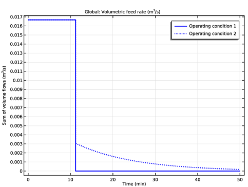
In the Settings window for Global, click Replace Expression in the upper-right corner of the y-Axis Data section. From the menu, choose Component 1 (comp1)>Reaction Engineering>re.sumvf - Sum of volume flows - m³/s.
|
|
3
|
|
4
|
|
5
|
|
6
|
|
7
|
|
8
|
Click to expand the Coloring and Style section. Find the Line style subsection. From the Line list, choose Cycle.
|
|
9
|
|
10
|
|
11
|
|
13
|
|
1
|
|
2
|
|
3
|
|
4
|
|
1
|
|
2
|
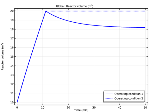
In the Settings window for Global, click Replace Expression in the upper-right corner of the y-Axis Data section. From the menu, choose Component 1 (comp1)>Reaction Engineering>re.Vr - Reactor volume - m³.
|
|
3
|
|
4
|
|
5
|
|
6
|
Locate the Coloring and Style section. Find the Line style subsection. From the Line list, choose Cycle.
|
|
7
|
|
8
|
|
9
|
|
11
|
|
1
|
|
2
|
|
3
|
|
1
|
|
2
|
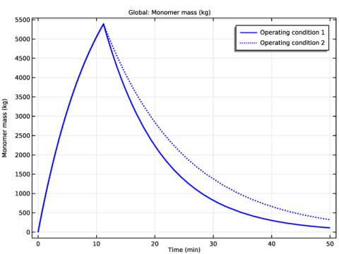
In the Settings window for Global, click Replace Expression in the upper-right corner of the y-Axis Data section. From the menu, choose Component 1 (comp1)>Definitions>Variables>m_mon - Monomer mass - kg.
|
|
3
|
|
4
|
|
5
|
|
6
|
Locate the Coloring and Style section. Find the Line style subsection. From the Line list, choose Cycle.
|
|
7
|
|
8
|
|
9
|
|
11
|