PDF

Syngas Combustion in a Round-Jet Burner
Introduction
This model simulates turbulent combustion of syngas (synthesis gas) in a simple round jet burner. Syngas is a gas mixture, primarily composed of hydrogen, carbon monoxide and carbon dioxide. The name syngas relates to its use in creating synthetic natural gas.
The model setup corresponds to the one studied by Couci and others in Ref. 1. The temperature and composition resulting from the nonpremixed combustion in the burner setup have also been experimentally investigated by Barlow and coworkers (Ref. 2 and Ref. 3) as a part of the International Workshop on Measurement and Computation of Turbulent Nonpremixed Flames (Ref. 4). The model is solved in COMSOL Multiphysics by combining a Reacting Flow and a Heat Transfer in Fluids interface.
Model Definition
The burner studied in this model consists of a straight pipe placed in a slight coflow. The gas phase fuel is fed through the pipe using an inlet velocity of 76 m/s, while the coflow velocity outside of pipe is 0.7 m/s. At the pipe exit, the fuel gas mixes with the coflow, creating an unconfined circular jet. The gas fed through the tube consists of three compounds typical of syngas: carbon monoxide (CO), hydrogen (H2), and nitrogen (N2). The coflow gas consists of air. At the pipe exit, the fuel is ignited. Since the fuel and oxidizer enter the reaction zone separately, the resulting combustion is of the nonpremixed type. A continuous reaction requires that the reactants and the oxidizer are mixed to stoichiometric conditions. In this setup, the turbulent flow of the jet effectively mixes the fuel from the pipe with the coflowing oxygen. Furthermore, the mixture needs to be continuously ignited. In this burner the small recirculation zones generated by the pipe wall thickness provide the means to decelerate hot product gas. The recirculation zones hereby promote continuous ignition of the oncoming mixture and stabilizes the flame at the pipe orifice. In experiments (Ref. 4), no lift-off or localized extinction of the flame has been observed.
In the current model, the syngas combustion is modeled using two irreversible reactions:
(1)
This assumption of a complete oxidation of the fuel corresponds to one of the approaches used in Ref. 1. The mass transport in the reacting jet is modeled by solving for the mass fractions of six species: the five species participating in the reactions and nitrogen N2 originating in the coflowing air.
The Reynolds number for the jet, based on the inlet velocity and the inner diameter of the pipe, is approximately 16,700, indicating that the jet is fully turbulent. Under these circumstances, both the mixing and the reactions processes in the jet are significantly influenced by the turbulent nature of the flow. To account for the turbulence when solving for the flow field, the k-ω turbulence model is applied.
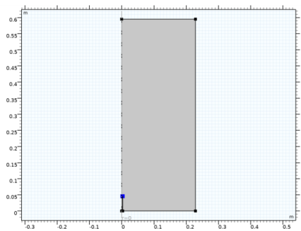
Taking advantage of the symmetry, a two-dimensional model using a cylindrical coordinate system is solved.
Turbulent reaction rate
When using a turbulence model in a Reacting Flow interface, the production rate (SI unit: kg/(m3·s)) of species i resulting from reaction j is modeled as the minimum of the mean-value-closure reaction rate and the eddy-dissipation-model rate:
The mean-value-closure rate is the kinetic reaction rate expressed using the mean mass fractions. This corresponds to the characteristic reaction rate for reactions that are slow compared to the turbulent mixing, or the reaction rate in regions with negligible turbulence levels. This can be quantified through the Damköhler number, which compares the turbulent time scale (τT) to the chemical time scale (τc). The mean-value-closure is appropriate for low Damköhler numbers:
The reaction rate defined by the eddy-dissipation model (Ref. 5) is:
(2)
where τT (SI unit: s) is the mixing time scale of the turbulence, ρ is the mixture density (SI unit: kg/m3), ω is the species mass fraction, ν denotes the stoichiometric coefficients, and M is the molar mass (SI unit: kg/mol). Properties of reactants of the reaction are indicated using a subscript r, while product properties are denoted by a subscript p.
The eddy-dissipation model assumes that both the Reynolds and Damköhler numbers are sufficiently high for the reaction rate to be limited by the turbulent mixing time scale τT. A global reaction can then at most progress at the rate at which fresh reactants are mixed, at the molecular level, by the turbulence present. The reaction rate is also assumed to be limited by the deficient reactant; the reactant with the lowest local concentration. The model parameter β specifies that product species is required for reaction, modeling the activation energy. For gaseous non-premixed combustion the model parameters have been found to be (Ref. 5):
,
In the current model the molecular reaction rate of the reactions is assumed to be infinitely fast. This is achieved in the model by prescribing unrealistically high rate constants for the reactions. This implies that the production rate is given solely by the turbulent mixing in Equation 2.
It should be noted that the eddy-dissipation model is a robust but simple model for turbulent reactions. The reaction rate is governed by a single time scale, the turbulent mixing time-scale. For this reason, the reactions studied should be limited to global one-step (as in Equation 1) or two-step reactions.
Heat of reaction
The heat of reaction, or change in enthalpy, following each reaction is defined from the heat of formation of the products and reactants:
The heat of formations for each species is given in Table 1 (based on Ref. 6). Since the heat of formation of the products is lower than that of the reactants, both reactions are exothermic and release heat. The heat release is included in the model by adding a Heat Source feature to the Heat Transfer in Fluids interface. The heat source (SI unit: W/m3) applied is defined as:
 
ΔHf (cal/mol)
Cp (cal/(mol·K)
Cp (cal/(mol·K)
Cp (cal/(mol·K)
N2
H2
O2
H2O
Heat capacity
The temperature in the jet increases significantly due to the heat release following the reactions, this is one of the defining features of combustion. For an accurate prediction of the temperature it is important to account for the temperature dependence of the species heat capacities. In the model, interpolation functions for the heat capacity at constant pressure, Cp,i (SI unit: cal/(mol·K)), for each species are defined using the values at three different temperatures given in Table 1. The heat capacity of the mixture, cp,mix (SI unit: J/(kg·K)), is computed as a mass fraction weighted mean of the individual heat capacities:
Results and Discussion
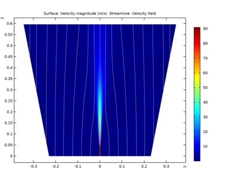
The resulting velocity field in the nonisothermal reacting jet is visualized in Figure 1. The expansion and development of the hot free jet is clearly seen. The turbulent mixing in the outer parts of the jet acts to accelerate fluid originating in the co-flow, and incorporate it in the jet. This is commonly referred to as entrainment and can be observed in the co-flow streamlines which bend toward the jet downstream of the orifice.
Figure 1: The velocity magnitude and flow paths (streamlines) of the reacting jet.
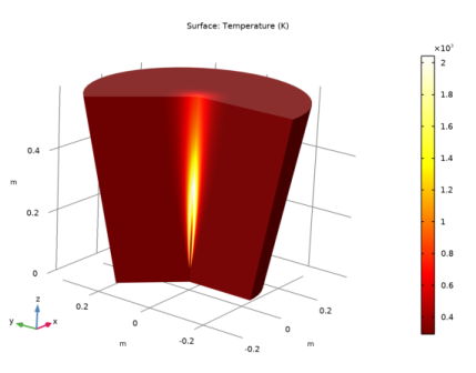
The temperature in the jet is shown in Figure 2 where a revolved dataset has been used to emphasize the structure of the round jet. The maximum temperature in the jet is seen to be approximately 2040 K. The carbon dioxide mass fraction in the reacting jet is plotted in Figure 3. The formation of CO2 takes place in the outer shear layer of the jet. This is where the fuel from the pipe encounters oxygen in the coflow and reacts. The reactions are promoted by the turbulent mixing in the jet shear layer. It is also seen that the CO2 formation starts just outside of the pipe. This is also the case for the temperature increase in Figure 2. This implies that there is no lift-off and the flame is attached to the pipe.
In Figure 4, Figure 5, and Figure 6 the results reached in the model are compared with the experimental results of Barlow and coworkers (Ref. 2, Ref. 3, and Ref. 4). In Figure 4 the jet temperature is further examined and compared with the experiments. In the left panel the temperature along the centerline is plotted. It is seen that the maximum temperature predicted in the model is close to that in the experiment. However in the model the temperature profile is shifted in the downstream direction. This is most likely due to the fact that radiation has not been included in the model.
In the right panel of Figure 4 temperature profiles at 20 and 50 pipe diameters downstream of the pipe exit are compared with the experiments. The axial velocity of the jet is compared with the experimental results in Figure 5, using the same down stream positions. The axial velocity is found to compare well with the experimental values at both positions.
In Figure 6 the species concentration along the jet centerline is analyzed and compared with the experimental results. For some species, N2, and CO2, the axial mass fraction development agrees well with the experimental results. For the fuel species CO and H2 a fair agreement is observed. For the remaining species, O2 and H2O, the trend appears correct but the profiles are shifted downstream, as was the case with the temperature. The reason for the discrepancy in the mass fractions can in part be attributed to the fact that radiation is not included, but the accuracy is probably also significantly influenced by the simplified reaction scheme and the eddy-dissipation model.
Figure 2: Jet temperature shown using a revolved dataset.
Figure 3: CO2 mass fraction in the reacting jet.
Figure 4: Jet temperature along the centerline (left), and radially at two different positions downstream of the pipe exit (right) scaled by the inlet temperature. The centerline and radial distance is scaled by the inner diameter of the pipe. Model results are plotted using lines, while experimental results are indicated using symbols. The downstream positions are defined in terms of the inner diameter of the pipe (d).
Figure 5: Axial velocity at two different positions downstream of the pipe exit, scaled by the inlet velocity. The radial distance is scaled by the inner diameter of the pipe. Model results are plotted using lines, while experimental results are indicated using symbols.
Figure 6: Species mass fractions along the jet centerline. The centerline distance is scaled by the inner diameter of the pipe. Model results are plotted using lines, while experimental results are indicated using symbols.
References
1. A. Cuoci, A. Frassoldati, G. Buzzi Ferraris, T. Faravelli, E. Ranzi, “The ignition, combustion and flame structure of carbon monoxide/hydrogen mixtures. Note 2: Fluid dynamics and kinetic aspects of syngas combustion,” Int. J. Hydrogen Energy, vol. 32, pp. 3486–3500, 2007
2. R.S. Barlow, G.J. Fiechtner, C.D. Carter, and J.-Y. Chen, “Experiments on the Scalar Structure of Turbulent CO/H2/N2 Jet Flames,” Comb. and Flame, vol. 120, pp. 549–569, 2000.
3. M. Flury, Experimentelle Analyse der Mischungstruktur in turbulenten nicht vorgemischten Flammen, Ph.D. Thesis, ETH Zurich, 1998.
4. R.S. Barlow and others, “Sandia/ETH-Zurich CO/H2/N2 Flame Data - Release 1.1,” http://www.sandia.gov/TNF/DataArch/SANDchnWeb/SANDchnDoc11.pdf, 2002.
5. B.F. Magnussen and B.H. Hjertager, “On Mathematical Modeling of Turbulent Combustion with Special Emphasis on Soot Formation and Combustion,” 16th Symp. (Int.) on Combustion. Comb. Inst., Pittsburg, Pennsylvania, pp.719–729, 1976.
6. A. Frassoldati, T. Faravelli, and E. Ranzi, “The Ignition, Combustion and Flame Structure of Carbon Monoxide/Hydrogen Mixtures. Note 1: Detailed Kinetic Modeling of Syngas Combustion Also in Presence of Nitrogen Compounds,” Int. J. Hydrogen Energy, vol. 32, pp. 3471–3485, 2007.
Application Library path: Chemical_Reaction_Engineering_Module/Reactors_with_Mass_and_Heat_Transfer/round_jet_burner
Modeling Instructions
From the File menu, choose New.
New
In the New window, click  Blank Model.
Global Definitions
Parameters 1
1
In the Model Builder window, under Global Definitions click Parameters 1.
2
In the Settings window for Parameters, locate the Parameters section.
3
Click  Load from File.
4
Add Component
In the Home toolbar, click  Add Component and choose 2D Axisymmetric.
Add Physics
1
In the Home toolbar, click  Add Physics to open the Add Physics window.
2
Go to the Add Physics window.
3
In the tree, select Chemical Species Transport>Reacting Flow>Turbulent Flow>Turbulent Flow, k-ω.
4
Click to expand the Dependent Variables section. In the Number of species text field, type 6.
5
In the Mass fractions table, enter the following settings:
6
Click Add to Component 1 in the window toolbar.
7
In the tree, select Heat Transfer>Heat Transfer in Fluids (ht).
8
Click Add to Component 1 in the window toolbar.
9
In the Home toolbar, click  Add Physics to close the Add Physics window.
Add Multiphysics
1
In the Home toolbar, click  Add Multiphysics to open the Add Multiphysics window.
2
Go to the Add Multiphysics window.
3
In the tree, select No Predefined Multiphysics Available for the Selected Physics Interfaces.
4
Find the Select the physics interfaces you want to couple subsection. In the table, clear the Couple check box for Transport of Concentrated Species (tcs).
5
In the tree, select Fluid Flow>Nonisothermal Flow>Turbulent Flow>Turbulent Flow, k-ω.
6
Click Add to Component in the window toolbar.
7
In the Home toolbar, click  Add Multiphysics to close the Add Multiphysics window.
Multiphysics
Nonisothermal Flow 1 (nitf1)
1
In the Settings window for Nonisothermal Flow, locate the Material Properties section.
2
From the Specify density list, choose Custom.
3
From the ρ list, choose Density (tcs/cdm1).
Add Study
1
In the Home toolbar, click  Add Study to open the Add Study window.
2
Go to the Add Study window.
3
Find the Studies subsection. In the Select Study tree, select General Studies>Stationary.
4
Click Add Study in the window toolbar.
5
In the Home toolbar, click  Add Study to close the Add Study window.
Definitions
Variables 1
1
In the Home toolbar, click  Variables and choose Local Variables.
2
In the Settings window for Variables, locate the Variables section.
3
Click  Load from File.
4
Geometry 1
Rectangle 1 (r1)
1
In the Geometry toolbar, click  Rectangle.
2
In the Settings window for Rectangle, locate the Size and Shape section.
3
In the Width text field, type GeomW.
4
In the Height text field, type GeomH.
5
Click  Build Selected.
Rectangle 2 (r2)
1
In the Geometry toolbar, click  Rectangle.
2
In the Settings window for Rectangle, locate the Size and Shape section.
3
In the Width text field, type Pth.
4
In the Height text field, type Pl.
5
Locate the Position section. In the r text field, type Di/2.
6
Click  Build Selected.
Chamfer 1 (cha1)
1
In the Geometry toolbar, click  Chamfer.
2
On the object r2, select Points 3 and 4 only.
It might be easier to select the points by using the Selection List window. To open this window, in the Home toolbar click Windows and choose Selection List. (If you are running the cross-platform desktop, you find Windows in the main menu.)
3
In the Settings window for Chamfer, locate the Distance section.
4
In the Distance from vertex text field, type Pth*0.15.
5
Click  Build Selected.
6
Click the  Zoom Extents button in the Graphics toolbar.
Polygon 1 (pol1)
1
In the Geometry toolbar, click  Polygon.
2
In the Settings window for Polygon, locate the Coordinates section.
3
From the Data source list, choose Vectors.
4
In the r text field, type GeomW GeomW*1.5 GeomW*1.5 GeomW.
5
In the z text field, type 0 GeomH GeomH GeomH.
6
Click  Build Selected.
Union 1 (uni1)
1
In the Geometry toolbar, click  Booleans and Partitions and choose Union.
2
Select the objects pol1 and r1 only.
3
In the Settings window for Union, locate the Union section.
4
Clear the Keep interior boundaries check box.
5
Click  Build Selected.
Difference 1 (dif1)
1
In the Geometry toolbar, click  Booleans and Partitions and choose Difference.
2
3
In the Settings window for Difference, locate the Difference section.
4
Find the Objects to subtract subsection. Select the  Activate Selection toggle button.
5
6
Click  Build Selected.
Line Segment 1 (ls1)
1
In the Geometry toolbar, click  More Primitives and choose Line Segment.
2
In the Settings window for Line Segment, locate the Starting Point section.
3
From the Specify list, choose Coordinates.
4
Locate the Endpoint section. From the Specify list, choose Coordinates.
5
In the r text field, type Di/2.
6
Locate the Starting Point section. In the z text field, type Pl-0.15*Pth.
7
Locate the Endpoint section. In the z text field, type Pl-0.15*Pth.
8
Click  Build Selected.
Line Segment 2 (ls2)
1
In the Geometry toolbar, click  More Primitives and choose Line Segment.
2
In the Settings window for Line Segment, locate the Starting Point section.
3
From the Specify list, choose Coordinates.
4
Locate the Endpoint section. From the Specify list, choose Coordinates.
5
Locate the Starting Point section. In the r text field, type Di/2+Pth.
6
Locate the Endpoint section. In the r text field, type GeomW+0.5*(Pl-0.15*Pth)*GeomW/GeomH.
7
Locate the Starting Point section. In the z text field, type Pl-0.15*Pth.
8
Locate the Endpoint section. In the z text field, type Pl-0.15*Pth.
9
Click  Build Selected.
Line Segment 3 (ls3)
1
In the Geometry toolbar, click  More Primitives and choose Line Segment.
2
In the Settings window for Line Segment, locate the Starting Point section.
3
From the Specify list, choose Coordinates.
4
Locate the Endpoint section. From the Specify list, choose Coordinates.
5
Locate the Starting Point section. In the r text field, type Di/2.
6
Locate the Endpoint section. In the r text field, type Di/2+(GeomH-Pl+Pth*0.15)*tan(pi/180).
7
Locate the Starting Point section. In the z text field, type Pl-0.15*Pth.
8
Locate the Endpoint section. In the z text field, type GeomH.
9
Click  Build Selected.
Line Segment 4 (ls4)
1
In the Geometry toolbar, click  More Primitives and choose Line Segment.
2
In the Settings window for Line Segment, locate the Starting Point section.
3
From the Specify list, choose Coordinates.
4
Locate the Endpoint section. From the Specify list, choose Coordinates.
5
Locate the Starting Point section. In the r text field, type Di/2+Pth.
6
Locate the Endpoint section. In the r text field, type Di/2+Pth+(GeomH-Pl+Pth*0.15)*tan(5*pi/180).
7
Locate the Starting Point section. In the z text field, type Pl-0.15*Pth.
8
Locate the Endpoint section. In the z text field, type GeomH.
9
Click  Build Selected.
Form Union (fin)
1
In the Model Builder window, click Form Union (fin).
2
In the Settings window for Form Union/Assembly, click  Build Selected.
Mesh Control Edges 1 (mce1)
1
In the Geometry toolbar, click  Virtual Operations and choose Mesh Control Edges.
2
On the object fin, select Boundaries 4, 8, 13, and 14 only.
3
In the Settings window for Mesh Control Edges, click  Build Selected.
4
Click the  Zoom Extents button in the Graphics toolbar.
Form Composite Edges 1 (cme1)
1
In the Geometry toolbar, click  Virtual Operations and choose Form Composite Edges.
2
On the object mce1, select Boundaries 3 and 11 only.
3
In the Settings window for Form Composite Edges, click  Build Selected.
Turbulent Flow, k-ω (spf)
Fluid Properties 1
1
In the Model Builder window, under Component 1 (comp1)>Turbulent Flow, k-ω (spf) click Fluid Properties 1.
2
In the Settings window for Fluid Properties, locate the Fluid Properties section.
3
From the μ list, choose User defined. In the associated text field, type mu_mix.
Inlet 1
1
In the Physics toolbar, click  Boundaries and choose Inlet.
2
3
In the Settings window for Inlet, locate the Boundary Condition section.
4
From the list, choose Fully developed flow.
Inlet 2
In the Physics toolbar, click  Boundaries and choose Inlet.
Inlet 1
1
In the Model Builder window, click Inlet 1.
2
In the Settings window for Inlet, locate the Fully Developed Flow section.
3
In the Uav text field, type Ujet.
Inlet 2
1
In the Model Builder window, click Inlet 2.
2
3
In the Settings window for Inlet, locate the Velocity section.
4
Click the Velocity field button.
5
Specify the u0 vector as
6
Locate the Turbulence Conditions section. From the IT list, choose Low (0.01).
7
From the LT list, choose User defined.
8
Outlet 1
1
In the Physics toolbar, click  Boundaries and choose Outlet.
2
3
In the Settings window for Outlet, locate the Pressure Conditions section.
4
Select the Normal flow check box.
Transport of Concentrated Species (tcs)
1
In the Model Builder window, under Component 1 (comp1) click Transport of Concentrated Species (tcs).
2
In the Settings window for Transport of Concentrated Species, locate the Transport Mechanisms section.
3
From the Diffusion model list, choose Fick’s law.
4
Locate the Species section. From the From mass constraint list, choose wN2.
Transport Properties 1
Apply the temperature from the heat transfer interface.
1
In the Model Builder window, under Component 1 (comp1)>Transport of Concentrated Species (tcs) click Transport Properties 1.
2
In the Settings window for Transport Properties, locate the Model Input section.
3
From the T list, choose Temperature (ht).
4
Locate the Density section. In the MwCO text field, type M_CO.
5
In the MwO2 text field, type M_O2.
6
In the MwCO2 text field, type M_CO2.
7
In the MwH2 text field, type M_H2.
8
In the MwH2O text field, type M_H2O.
9
In the MwN2 text field, type M_N2.
Initial Values 1
1
In the Model Builder window, click Initial Values 1.
2
In the Settings window for Initial Values, locate the Initial Values section.
3
In the ω0,wCO text field, type 0.
4
In the ω0,wO2 text field, type wcf_O2.
5
In the ω0,wCO2 text field, type 0.
6
In the ω0,wH2 text field, type 0.
7
In the ω0,wH2O text field, type 0.
Inflow 1
1
In the Physics toolbar, click  Boundaries and choose Inflow.
2
3
In the Settings window for Inflow, locate the Inflow section.
4
From the Mixture specification list, choose Mole fractions.
5
In the x0,wCO text field, type x0_CO.
6
In the x0,wO2 text field, type x0_O2.
7
In the x0,wCO2 text field, type x0_CO2.
8
In the x0,wH2 text field, type x0_H2.
9
In the x0,wH2O text field, type x0_H2O.
Inflow 2
1
In the Physics toolbar, click  Boundaries and choose Inflow.
2
3
In the Settings window for Inflow, locate the Inflow section.
4
In the ω0,wCO text field, type 1e-5.
5
In the ω0,wO2 text field, type wcf_O2.
6
In the ω0,wCO2 text field, type 1e-5.
7
In the ω0,wH2 text field, type 1e-5.
8
In the ω0,wH2O text field, type 1e-5.
Outflow 1
1
In the Physics toolbar, click  Boundaries and choose Outflow.
2
Reaction 1
1
In the Physics toolbar, click  Domains and choose Reaction.
2
3
In the Settings window for Reaction, locate the Reaction Rate section.
4
In the νwCO text field, type -1.
5
In the νwO2 text field, type -0.5.
6
In the νwCO2 text field, type 1.
Apply an unrealistically high reaction rate to model the reactions as infinitely fast. In this case the reaction rate will be given by the turbulent mixing.
7
Locate the Rate Constants section. In the kf text field, type 1e100.
8
Locate the Turbulent Flow section. From the Turbulent-reaction model list, choose Eddy-dissipation.
Regularization makes the reaction system much easier to converge.
9
Click to expand the Regularization section. Select the Rate expressions check box.
Reaction 2
1
Right-click Reaction 1 and choose Duplicate.
2
In the Settings window for Reaction, locate the Reaction Rate section.
3
In the νwCO text field, type 0.
4
In the νwCO2 text field, type 0.
5
In the νwH2 text field, type -1.
6
In the νwH2O text field, type 1.
Use the tabulated heat capacities to create interpolation functions, one for each species.
Definitions
Interpolation 1 (int1)
1
In the Home toolbar, click  Functions and choose Local>Interpolation.
2
In the Settings window for Interpolation, locate the Definition section.
3
In the Function name text field, type Cp_CO.
4
5
Locate the Interpolation and Extrapolation section. From the Interpolation list, choose Piecewise cubic.
6
Locate the Units section. In the Arguments text field, type K.
7
In the Function text field, type cal/mol/K.
Plot the resulting interpolation function.
8
Interpolation 2 (Cp_CO2)
1
Right-click Interpolation 1 (int1) and choose Duplicate.
2
In the Settings window for Interpolation, locate the Definition section.
3
In the Function name text field, type Cp_CO2.
4
Interpolation 3 (Cp_CO3)
1
Right-click Interpolation 2 (Cp_CO2) and choose Duplicate.
2
In the Settings window for Interpolation, locate the Definition section.
3
In the Function name text field, type Cp_H2.
4
Interpolation 4 (Cp_H3)
1
Right-click Interpolation 3 (Cp_CO3) and choose Duplicate.
2
In the Settings window for Interpolation, locate the Definition section.
3
In the Function name text field, type Cp_H2O.
4
Interpolation 5 (Cp_H2O2)
1
Right-click Interpolation 4 (Cp_H3) and choose Duplicate.
2
In the Settings window for Interpolation, locate the Definition section.
3
In the Function name text field, type Cp_N2.
4
Interpolation 6 (Cp_N3)
1
Right-click Interpolation 5 (Cp_H2O2) and choose Duplicate.
2
In the Settings window for Interpolation, locate the Definition section.
3
In the Function name text field, type Cp_O2.
4
Define the mixture heat capacity. It is computed as the mass average of the species capacities. Also define the enthalpy change for each of the reactions included.
Variables 1
1
In the Model Builder window, click Variables 1.
2
In the Settings window for Variables, locate the Variables section.
3
Now setup the heat transfer interface.
Heat Transfer in Fluids (ht)
Fluid 1
1
In the Model Builder window, under Component 1 (comp1)>Heat Transfer in Fluids (ht) click Fluid 1.
2
In the Settings window for Fluid, locate the Heat Conduction, Fluid section.
3
From the k list, choose User defined. In the associated text field, type k_mix.
4
Locate the Thermodynamics, Fluid section. From the Specify Cp or γ list, choose Ideal gas: heat capacity at constant pressure.
5
From the Cp list, choose User defined. In the associated text field, type Cp_mix.
Initial Values 1
1
In the Model Builder window, click Initial Values 1.
2
In the Settings window for Initial Values, locate the Initial Values section.
3
In the T text field, type T0.
Inflow 1
1
In the Physics toolbar, click  Boundaries and choose Inflow.
2
3
In the Settings window for Inflow, locate the Upstream Properties section.
4
In the Tustr text field, type T0.
Outflow 1
1
In the Physics toolbar, click  Boundaries and choose Outflow.
2
Heat Source 1
1
In the Physics toolbar, click  Domains and choose Heat Source.
2
3
In the Settings window for Heat Source, locate the Heat Source section.
4
In the Q0 text field, type -(dH_R1*tcs.treac1.r+dH_R2*tcs.treac2.r).
Mesh 1
Mapped 1
1
In the Mesh toolbar, click  Mapped.
2
In the Settings window for Mapped, click to expand the Control Entities section.
3
Clear the Smooth across removed control entities check box.
Distribution 1
1
Right-click Mapped 1 and choose Distribution.
2
3
In the Settings window for Distribution, locate the Distribution section.
4
From the Distribution type list, choose Predefined.
5
In the Number of elements text field, type 20.
6
In the Element ratio text field, type 4.
7
From the Growth formula list, choose Geometric sequence.
Distribution 2
1
In the Model Builder window, right-click Mapped 1 and choose Distribution.
2
3
In the Settings window for Distribution, locate the Distribution section.
4
From the Distribution type list, choose Predefined.
5
In the Number of elements text field, type 200.
6
In the Element ratio text field, type 250.
7
From the Growth formula list, choose Geometric sequence.
Distribution 3
1
Right-click Mapped 1 and choose Distribution.
2
3
In the Settings window for Distribution, locate the Distribution section.
4
From the Distribution type list, choose Predefined.
5
In the Number of elements text field, type 20.
6
In the Element ratio text field, type 400.
7
From the Growth formula list, choose Geometric sequence.
8
Select the Reverse direction check box.
Distribution 4
1
Right-click Mapped 1 and choose Distribution.
2
3
In the Settings window for Distribution, locate the Distribution section.
4
From the Distribution type list, choose Predefined.
5
In the Number of elements text field, type 20.
6
In the Element ratio text field, type 200.
7
From the Growth formula list, choose Geometric sequence.
8
Select the Reverse direction check box.
Distribution 5
1
Right-click Mapped 1 and choose Distribution.
2
3
In the Settings window for Distribution, locate the Distribution section.
4
From the Distribution type list, choose Predefined.
5
In the Number of elements text field, type 20.
6
In the Element ratio text field, type 8.
7
From the Growth formula list, choose Geometric sequence.
Distribution 6
1
Right-click Mapped 1 and choose Distribution.
2
3
In the Settings window for Distribution, locate the Distribution section.
4
From the Distribution type list, choose Predefined.
5
In the Number of elements text field, type 20.
6
In the Element ratio text field, type 4.
7
From the Growth formula list, choose Geometric sequence.
8
Click  Build All.
Study 1
Solution 1 (sol1)
1
In the Study toolbar, click  Show Default Solver.
2
In the Model Builder window, expand the Solution 1 (sol1) node.
3
In the Model Builder window, expand the Study 1>Solver Configurations>Solution 1 (sol1)>Stationary Solver 1 node.
4
In the Model Builder window, under Study 1>Solver Configurations>Solution 1 (sol1)>Stationary Solver 1 click Segregated 1.
5
In the Settings window for Segregated, locate the General section.
6
In the PID controller - proportional text field, type 0.65.
7
In the PID controller - derivative text field, type 0.025.
8
In the Target error estimate text field, type 0.1.
9
In the Model Builder window, under Study 1>Solver Configurations>Solution 1 (sol1)>Stationary Solver 1>Segregated 1 click Velocity u, Pressure p.
10
In the Settings window for Segregated Step, locate the General section.
11
Under Variables, click  Add.
12
In the Add dialog box, in the Variables list, choose Wall temperature, downside (comp1.nitf1.TWall_d), Wall temperature, upside (comp1.nitf1.TWall_u), and Temperature (comp1.T).
13
14
In the Model Builder window, under Study 1>Solver Configurations>Solution 1 (sol1)>Stationary Solver 1>Segregated 1 click Mass fractions.
15
In the Settings window for Segregated Step, click to expand the Method and Termination section.
16
In the Number of iterations text field, type 2.
17
In the Damping factor text field, type 0.4.
18
In the Model Builder window, under Study 1>Solver Configurations>Solution 1 (sol1)>Stationary Solver 1>Segregated 1 right-click Temperature and choose Disable.
Solution 1 (sol1)
1
In the Model Builder window, collapse the Study 1>Solver Configurations>Solution 1 (sol1) node.
2
In the Model Builder window, right-click Solution 1 (sol1) and choose Compute.
Now move on to postprocess the result from the nonisothermal jet. Start by creating a mirrored 2D dataset as well as a revolved 3D dataset.
Results
Mirror 2D 1
In the Results toolbar, click  More Datasets and choose Mirror 2D.
Cut Line 2D 1
1
In the Results toolbar, click  Cut Line 2D.
2
In the Settings window for Cut Line 2D, locate the Data section.
3
From the Dataset list, choose Mirror 2D 1.
4
Locate the Line Data section. From the Line entry method list, choose Point and direction.
5
Find the Point subsection. In the y text field, type Pl+20*Di.
6
Click to expand the Advanced section. Find the Space variable subsection. In the x text field, type r_mirr20.
Cut Line 2D 2
1
In the Results toolbar, click  Cut Line 2D.
2
In the Settings window for Cut Line 2D, locate the Data section.
3
From the Dataset list, choose Mirror 2D 1.
4
Locate the Line Data section. From the Line entry method list, choose Point and direction.
5
Find the Point subsection. In the y text field, type Pl+50*Di.
6
Locate the Advanced section. Find the Space variable subsection. In the x text field, type r_mirr50.
Now apply the mirror dataset to the existing plot groups.
Velocity (spf)
1
In the Model Builder window, click Velocity (spf).
2
In the Settings window for 2D Plot Group, locate the Data section.
3
From the Dataset list, choose Mirror 2D 1.
4
In the Velocity (spf) toolbar, click  Plot.
Streamline 1
Right-click Velocity (spf) and choose Streamline.
Streamline 1
1
In the Model Builder window, expand the Results>Velocity (spf) node, then click Streamline 1.
2
In the Settings window for Streamline, locate the Streamline Positioning section.
3
From the Positioning list, choose Uniform density.
4
In the Separating distance text field, type 0.035.
5
Locate the Coloring and Style section. Find the Point style subsection. From the Color list, choose Gray.
6
In the Velocity (spf) toolbar, click  Plot.
7
Click the  Zoom Extents button in the Graphics toolbar.
Pressure (spf)
1
In the Model Builder window, click Pressure (spf).
2
In the Settings window for 2D Plot Group, locate the Data section.
3
From the Dataset list, choose Mirror 2D 1.
4
In the Pressure (spf) toolbar, click  Plot.
Wall Resolution (spf)
1
In the Model Builder window, click Wall Resolution (spf).
2
In the Settings window for 2D Plot Group, locate the Data section.
3
From the Dataset list, choose Mirror 2D 1.
4
In the Wall Resolution (spf) toolbar, click  Plot.
Mass fraction, CO2
1
In the Model Builder window, right-click Concentration, CO2 (tcs) and choose Duplicate.
2
In the Settings window for 2D Plot Group, type Mass fraction, CO2 in the Label text field.
3
Locate the Data section. From the Dataset list, choose Mirror 2D 1.
4
Locate the Plot Settings section. From the Color list, choose White.
Surface 1
1
In the Model Builder window, expand the Mass fraction, CO2 node, then click Surface 1.
2
In the Settings window for Surface, locate the Expression section.
3
In the Expression text field, type wCO2.
4
In the Mass fraction, CO2 toolbar, click  Plot.
5
Click the  Zoom Extents button in the Graphics toolbar.
Temperature, 3D (ht)
1
In the Model Builder window, click Temperature, 3D (ht).
2
In the Settings window for 3D Plot Group, locate the Plot Settings section.
3
Clear the Plot dataset edges check box.
Import the experimental data files. The files corresponds to the ones published online (Ref. 2) by R. Barlow and coworkers. The name of the model, round_jet_burner, has been prepended to the filenames.
Centerline data
1
In the Results toolbar, click  Table.
2
In the Settings window for Table, type Centerline data in the Label text field.
3
Locate the Data section. Click Import.
4
z/Di = 20, Radial Data
1
In the Results toolbar, click  Table.
2
In the Settings window for Table, type z/Di = 20, Radial Data in the Label text field.
3
Locate the Data section. Click Import.
4
z/Di = 50, Radial Data
1
In the Results toolbar, click  Table.
2
In the Settings window for Table, type z/Di = 50, Radial Data in the Label text field.
3
Locate the Data section. Click Import.
4
z/Di = 20, Radial Velocity Data
1
In the Results toolbar, click  Table.
2
In the Settings window for Table, type z/Di = 20, Radial Velocity Data in the Label text field.
3
Locate the Data section. Click Import.
4
z/Di = 50, Radial Velocity Data
1
In the Results toolbar, click  Table.
2
In the Settings window for Table, type z/Di = 50, Radial Velocity Data in the Label text field.
3
Locate the Data section. Click Import.
4
1D Plot Group 20
In the Results toolbar, click  1D Plot Group.
Line Graph 1
1
Right-click 1D Plot Group 20 and choose Line Graph.
2
3
In the Settings window for Line Graph, locate the y-Axis Data section.
4
In the Expression text field, type T/T0.
5
Locate the x-Axis Data section. From the Parameter list, choose Expression.
6
In the Expression text field, type (z-Pl)/Di.
7
Click to expand the Coloring and Style section. From the Color list, choose Black.
8
Click to expand the Legends section. Select the Show legends check box.
9
From the Legends list, choose Manual.
10
Table Graph 1
1
In the Model Builder window, right-click 1D Plot Group 20 and choose Table Graph.
2
In the Settings window for Table Graph, locate the Data section.
3
From the x-axis data list, choose r(mm).
4
From the Plot columns list, choose Manual.
5
In the Columns list, select T(K).
6
Click to expand the Preprocessing section. Find the x-axis column subsection. From the Preprocessing list, choose Linear.
7
In the Scaling text field, type 1/(Di*1000).
8
Find the y-axis columns subsection. From the Preprocessing list, choose Linear.
9
In the Scaling text field, type 1/T0.
10
Locate the Coloring and Style section. Find the Line style subsection. From the Line list, choose None.
11
From the Color list, choose Black.
12
Find the Line markers subsection. From the Marker list, choose Square.
13
From the Positioning list, choose In data points.
14
Click to expand the Legends section. Select the Show legends check box.
15
From the Legends list, choose Manual.
16
T @ centerline
1
In the Model Builder window, under Results click 1D Plot Group 20.
2
In the Settings window for 1D Plot Group, type T @ centerline in the Label text field.
3
Locate the Plot Settings section. Select the x-axis label check box.
4
5
Select the y-axis label check box.
6
7
Locate the Axis section. Select the Manual axis limits check box.
8
In the x minimum text field, type -10.
9
In the x maximum text field, type 120.
10
In the y minimum text field, type 0.5.
11
In the y maximum text field, type 8.
12
Click to expand the Title section. From the Title type list, choose Manual.
13
In the Title text area, type Temperature along the centerline.
14
In the T @ centerline toolbar, click  Plot.
1D Plot Group 21
1
In the Home toolbar, click  Add Plot Group and choose 1D Plot Group.
2
In the Settings window for 1D Plot Group, locate the Data section.
3
From the Dataset list, choose None.
Line Graph 1
1
Right-click 1D Plot Group 21 and choose Line Graph.
2
In the Settings window for Line Graph, locate the Data section.
3
From the Dataset list, choose Cut Line 2D 1.
4
Locate the y-Axis Data section. In the Expression text field, type T/T0.
5
Locate the x-Axis Data section. From the Parameter list, choose Expression.
6
In the Expression text field, type r_mirr20/Di.
7
Locate the Coloring and Style section. From the Color list, choose Black.
8
Locate the Legends section. Select the Show legends check box.
9
From the Legends list, choose Manual.
10
Line Graph 2
1
Right-click Line Graph 1 and choose Duplicate.
2
In the Settings window for Line Graph, locate the Data section.
3
From the Dataset list, choose Cut Line 2D 2.
4
Locate the x-Axis Data section. In the Expression text field, type r_mirr50/Di.
5
Locate the Coloring and Style section. Find the Line style subsection. From the Line list, choose Dashed.
6
Locate the Legends section. In the table, enter the following settings:
7
In the 1D Plot Group 21 toolbar, click  Plot.
Table Graph 1
1
In the Model Builder window, right-click 1D Plot Group 21 and choose Table Graph.
2
In the Settings window for Table Graph, locate the Data section.
3
From the Table list, choose z/Di = 20, Radial Data.
4
From the x-axis data list, choose r(mm).
5
From the Plot columns list, choose Manual.
6
In the Columns list, select T(K).
7
Locate the Preprocessing section. Find the x-axis column subsection. From the Preprocessing list, choose Linear.
8
In the Scaling text field, type 1/(Di*1000).
9
Find the y-axis columns subsection. From the Preprocessing list, choose Linear.
10
In the Scaling text field, type 1/T0.
11
Locate the Coloring and Style section. Find the Line style subsection. From the Line list, choose None.
12
From the Color list, choose Black.
13
Find the Line markers subsection. From the Marker list, choose Square.
14
From the Positioning list, choose In data points.
15
Locate the Legends section. Select the Show legends check box.
16
From the Legends list, choose Manual.
17
Table Graph 2
1
Right-click Table Graph 1 and choose Duplicate.
2
In the Settings window for Table Graph, locate the Data section.
3
From the Table list, choose z/Di = 50, Radial Data.
4
Locate the Coloring and Style section. Find the Line markers subsection. From the Marker list, choose Triangle.
5
Locate the Legends section. In the table, enter the following settings:
T @ z/Di = 20, 50
1
In the Model Builder window, under Results click 1D Plot Group 21.
2
In the Settings window for 1D Plot Group, type T @ z/Di = 20, 50 in the Label text field.
3
Locate the Title section. From the Title type list, choose Manual.
4
In the Title text area, type Temperature downstream of the pipe exit.
5
Locate the Plot Settings section. Select the x-axis label check box.
6
7
Select the y-axis label check box.
8
9
Locate the Axis section. Select the Manual axis limits check box.
10
In the x minimum text field, type -10.
11
In the x maximum text field, type 10.
12
In the y minimum text field, type 0.5.
13
In the y maximum text field, type 8.
14
In the T @ z/Di = 20, 50 toolbar, click  Plot.
uz @ z/Di = 20, 50
1
In the Model Builder window, right-click T @ z/Di = 20, 50 and choose Duplicate.
2
In the Settings window for 1D Plot Group, type uz @ z/Di = 20, 50 in the Label text field.
Line Graph 1
1
In the Model Builder window, expand the uz @ z/Di = 20, 50 node, then click Line Graph 1.
2
In the Settings window for Line Graph, locate the y-Axis Data section.
3
In the Expression text field, type w/Ujet.
Line Graph 2
1
In the Model Builder window, click Line Graph 2.
2
In the Settings window for Line Graph, locate the y-Axis Data section.
3
In the Expression text field, type w/Ujet.
Table Graph 1
1
In the Model Builder window, click Table Graph 1.
2
In the Settings window for Table Graph, locate the Data section.
3
From the x-axis data list, choose Fblgr.
4
From the Table list, choose z/Di = 20, Radial Velocity Data.
5
In the Columns list, select uz.
6
Locate the Preprocessing section. Find the y-axis columns subsection. In the Scaling text field, type 1/Ujet.
Table Graph 2
1
In the Model Builder window, click Table Graph 2.
2
In the Settings window for Table Graph, locate the Data section.
3
From the x-axis data list, choose Fblgr.
4
From the Table list, choose z/Di = 50, Radial Velocity Data.
5
In the Columns list, select uz.
6
Locate the Preprocessing section. Find the y-axis columns subsection. In the Scaling text field, type 1/Ujet.
uz @ z/Di = 20, 50
1
In the Model Builder window, click uz @ z/Di = 20, 50.
2
In the Settings window for 1D Plot Group, locate the Title section.
3
In the Title text area, type Axial velocity downstream of the pipe exit.
4
Locate the Plot Settings section. In the y-axis label text field, type uz/Ujet.
5
Locate the Axis section. In the y minimum text field, type -0.25.
6
In the y maximum text field, type 1.25.
7
In the uz @ z/Di = 20, 50 toolbar, click  Plot.
8
Locate the Title section. From the Title type list, choose None.
CO, N2 @ centerline
1
In the Model Builder window, right-click T @ centerline and choose Duplicate.
2
In the Settings window for 1D Plot Group, type CO, N2 @ centerline in the Label text field.
3
Locate the Title section. In the Title text area, type Mass fraction along the centerline.
4
Locate the Plot Settings section. In the y-axis label text field, type wCO, wN2.
5
Locate the Axis section. In the y minimum text field, type -0.05.
6
In the y maximum text field, type 1.
7
In the CO, N2 @ centerline toolbar, click  Plot.
8
Locate the Legend section. From the Position list, choose Middle right.
Line Graph 1
1
In the Model Builder window, expand the CO, N2 @ centerline node, then click Line Graph 1.
2
In the Settings window for Line Graph, locate the y-Axis Data section.
3
In the Expression text field, type wCO.
4
Locate the Legends section. In the table, enter the following settings:
Table Graph 1
1
In the Model Builder window, click Table Graph 1.
2
In the Settings window for Table Graph, locate the Data section.
3
In the Columns list, select YCO.
4
Locate the Preprocessing section. Find the y-axis columns subsection. In the Scaling text field, type 1.
5
Locate the Legends section. In the table, enter the following settings:
6
In the CO, N2 @ centerline toolbar, click  Plot.
Line Graph 2
1
In the Model Builder window, under Results>CO, N2 @ centerline right-click Line Graph 1 and choose Duplicate.
2
In the Settings window for Line Graph, locate the y-Axis Data section.
3
In the Expression text field, type wN2.
4
Locate the Coloring and Style section. Find the Line style subsection. From the Line list, choose Dashed.
5
Locate the Legends section. In the table, enter the following settings:
Table Graph 2
1
In the Model Builder window, under Results>CO, N2 @ centerline right-click Table Graph 1 and choose Duplicate.
2
In the Settings window for Table Graph, locate the Data section.
3
In the Columns list, select YN2.
4
Locate the Coloring and Style section. Find the Line markers subsection. From the Marker list, choose Triangle.
5
Locate the Legends section. In the table, enter the following settings:
6
In the CO, N2 @ centerline toolbar, click  Plot.
H2, H2O @ centerline
1
In the Model Builder window, right-click CO, N2 @ centerline and choose Duplicate.
2
In the Settings window for 1D Plot Group, type H2, H2O @ centerline in the Label text field.
Line Graph 1
1
In the Model Builder window, expand the H2, H2O @ centerline node, then click Line Graph 1.
2
In the Settings window for Line Graph, locate the y-Axis Data section.
3
In the Expression text field, type wH2.
4
Locate the Legends section. In the table, enter the following settings:
Table Graph 1
1
In the Model Builder window, click Table Graph 1.
2
In the Settings window for Table Graph, locate the Data section.
3
In the Columns list, select YH2.
4
Locate the Legends section. In the table, enter the following settings:
Line Graph 2
1
In the Model Builder window, click Line Graph 2.
2
In the Settings window for Line Graph, locate the y-Axis Data section.
3
In the Expression text field, type wH2O.
4
Locate the Legends section. In the table, enter the following settings:
Table Graph 2
1
In the Model Builder window, click Table Graph 2.
2
In the Settings window for Table Graph, locate the Data section.
3
In the Columns list, select YH2O.
4
Locate the Legends section. In the table, enter the following settings:
H2, H2O @ centerline
1
In the Model Builder window, click H2, H2O @ centerline.
2
In the Settings window for 1D Plot Group, locate the Plot Settings section.
3
In the y-axis label text field, type wH2, wH2O.
4
Locate the Axis section. In the y maximum text field, type 0.15.
5
In the y minimum text field, type -0.02.
6
Locate the Legend section. From the Position list, choose Upper right.
7
In the H2, H2O @ centerline toolbar, click  Plot.
O2, CO2 @ centerline
1
In the Model Builder window, right-click H2, H2O @ centerline and choose Duplicate.
2
In the Settings window for 1D Plot Group, type O2, CO2 @ centerline in the Label text field.
Line Graph 1
1
In the Model Builder window, expand the O2, CO2 @ centerline node, then click Line Graph 1.
2
In the Settings window for Line Graph, locate the y-Axis Data section.
3
In the Expression text field, type wO2.
4
Locate the Legends section. In the table, enter the following settings:
Table Graph 1
1
In the Model Builder window, click Table Graph 1.
2
In the Settings window for Table Graph, locate the Data section.
3
In the Columns list, select YO2.
4
Locate the Legends section. In the table, enter the following settings:
Line Graph 2
1
In the Model Builder window, click Line Graph 2.
2
In the Settings window for Line Graph, locate the y-Axis Data section.
3
In the Expression text field, type wCO2.
4
Locate the Legends section. In the table, enter the following settings:
Table Graph 2
1
In the Model Builder window, click Table Graph 2.
2
In the Settings window for Table Graph, locate the Data section.
3
In the Columns list, select YCO2.
4
Locate the Legends section. In the table, enter the following settings:
O2, CO2 @ centerline
1
In the Model Builder window, click O2, CO2 @ centerline.
2
In the Settings window for 1D Plot Group, locate the Plot Settings section.
3
In the y-axis label text field, type wO2, wCO2.
4
Locate the Axis section. In the y minimum text field, type -0.05.
5
In the y maximum text field, type 0.4.
6
In the O2, CO2 @ centerline toolbar, click  Plot.