|
|
|

|
1
|
|
2
|
|
3
|
Click Add.
|
|
4
|
Click
|
|
5
|
|
6
|
Click
|
|
1
|
|
2
|
|
3
|
|
4
|
Browse to the model’s Application Libraries folder and double-click the file protein_adsorption_parameters.txt.
|
|
1
|
|
2
|
|
3
|
|
4
|
|
1
|
In the Model Builder window, under Component 1 (comp1) right-click Definitions and choose Variables.
|
|
2
|
|
1
|
|
2
|
|
3
|
|
4
|
|
1
|
|
2
|
|
3
|
|
4
|
Click Apply.
|
|
5
|
|
1
|
|
2
|
|
3
|
|
4
|
Click Apply.
|
|
5
|
|
6
|
|
7
|
In the Settings window for Reaction Engineering, click to expand the Equilibrium Species Vector section.
|
|
8
|
|
9
|
Locate the Reactor section. Find the Mass balance subsection. From the Volumetric rate list, choose User defined.
|
|
10
|
|
11
|
|
1
|
|
2
|
In the Settings window for Initial Values, click to expand the Surface Species Initial Values section.
|
|
3
|
|
1
|
|
2
|
|
3
|
|
4
|
Locate the Feed Inlet Concentration section. In the Feed inlet concentration table, enter the following settings:
|
|
1
|
|
2
|
|
3
|
|
4
|
|
1
|
|
2
|
|
3
|
|
4
|
|
1
|
|
2
|
|
3
|
|
4
|
|
1
|
|
2
|
|
3
|
|
1
|
|
2
|
|
3
|
|
1
|
|
2
|
|
3
|
|
1
|
|
2
|
|
3
|
|
4
|
|
1
|
|
2
|
|
3
|
|
4
|
|
5
|
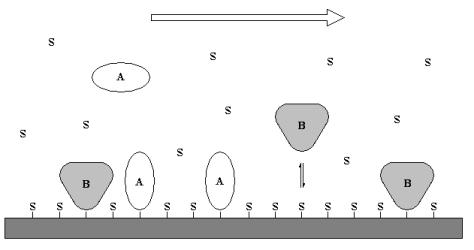
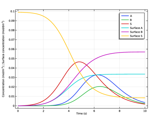
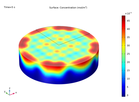
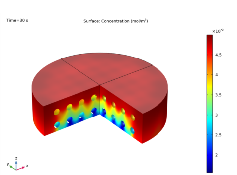
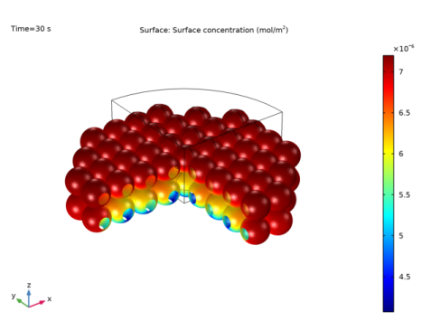
In the associated text field, type Concentration (mol/m<sup>-3</sup>) | Surface concentration (mol/dm<sup>-2</sup>).
|
|
1
|
|
2
|
In the Settings window for Global, click Replace Expression in the upper-right corner of the y-Axis Data section. From the menu, choose Component 1 (comp1)>Reaction Engineering>re.c_A - Concentration - mol/m³.
|
|
3
|
Click Add Expression in the upper-right corner of the y-Axis Data section. From the menu, choose Component 1 (comp1)>Reaction Engineering>re.c_B - Concentration - mol/m³.
|
|
4
|
Click Add Expression in the upper-right corner of the y-Axis Data section. From the menu, choose Component 1 (comp1)>Reaction Engineering>re.c_S - Concentration - mol/m³.
|
|
5
|
Click Add Expression in the upper-right corner of the y-Axis Data section. From the menu, choose Component 1 (comp1)>Reaction Engineering>re.csurf_A_surf - Surface concentration - mol/m².
|
|
6
|
Click Add Expression in the upper-right corner of the y-Axis Data section. From the menu, choose Component 1 (comp1)>Reaction Engineering>re.csurf_B_surf - Surface concentration - mol/m².
|
|
7
|
Click Add Expression in the upper-right corner of the y-Axis Data section. From the menu, choose Component 1 (comp1)>Reaction Engineering>re.csurf_S_surf - Surface concentration - mol/m².
|
|
8
|
|
9
|
|
10
|
|
12
|
|
1
|
|
2
|
|
3
|
|
4
|
|
5
|
|
6
|
|
1
|
|
2
|
|
4
|
|
5
|
In the Settings window for Reaction Engineering, click to expand the Calculate Transport Properties section.
|
|
6
|
|
7
|
|
8
|
|
1
|
|
2
|
|
3
|
|
4
|
Locate the Physics Interfaces section. Find the Fluid flow subsection. From the list, choose Laminar Flow: New.
|
|
5
|
|
1
|
|
2
|
|
3
|
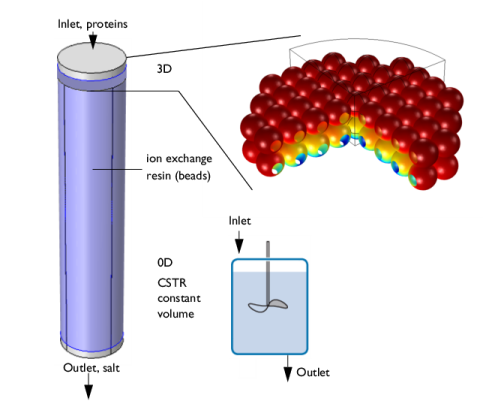
Browse to the model’s Application Libraries folder and double-click the file protein_adsorption_geom_sequence.mph.
|
|
4
|
|
5
|
|
1
|
In the Model Builder window, expand the Component 2 (comp2)>Transport of Diluted Species (tds) node, then click Inflow 1.
|
|
2
|
|
3
|
|
4
|
|
5
|
|
6
|
|
1
|
|
2
|
|
3
|
|
1
|
|
2
|
|
3
|
|
1
|
|
2
|
|
3
|
|
1
|
|
2
|
|
3
|
|
4
|
|
5
|
|
1
|
|
2
|
|
3
|
|
1
|
|
2
|
|
3
|
|
1
|
|
2
|
|
3
|
|
4
|
|
1
|
|
2
|
|
3
|
|
4
|
|
1
|
|
2
|
|
3
|
|
4
|
|
5
|
|
1
|
|
2
|
|
3
|
|
1
|
|
2
|
|
3
|
|
1
|
|
2
|
|
3
|
Click the Custom button.
|
|
4
|
|
1
|
|
2
|
|
3
|
|
4
|
|
1
|
|
2
|
|
3
|
Click the Custom button.
|
|
4
|
|
1
|
|
2
|
|
3
|
In the table, clear the Solve for check boxes for Reaction Engineering (re), Chemistry 1 (chem), Transport of Diluted Species (tds), and Surface Reactions 1 (sr).
|
|
1
|
|
2
|
|
3
|
|
4
|
|
5
|
|
6
|
Locate the Physics and Variables Selection section. In the table, clear the Solve for check box for Laminar Flow 1 (spf).
|
|
1
|
|
2
|
|
3
|
|
4
|
|
5
|
|
6
|
|
7
|
|
8
|
|
9
|
|
10
|
|
11
|
|
12
|
|
1
|
|
2
|
|
3
|
|
4
|
Click
|
|
1
|
|
2
|
|
3
|
|
4
|
|
5
|
|
6
|
Click
|
|
1
|
|
2
|
|
1
|
|
2
|
|
3
|
|
4
|
|
5
|
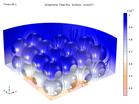
Click Replace Expression in the upper-right corner of the Expression section. From the menu, choose Component 2 (comp2)>Transport of Diluted Species>Species cB>cB - Concentration - mol/m³.
|
|
6
|
|
1
|
|
2
|
|
3
|
|
4
|
|
5
|
|
1
|
|
2
|
|
3
|
|
4
|
|
1
|
|
2
|
|
3
|
|
4
|
|
5
|
|
1
|
|
2
|
|
1
|
|
2
|
|
3
|
|
4
|
|
5
|
Click Replace Expression in the upper-right corner of the Expression section. From the menu, choose Component 2 (comp2)>Surface Reactions 1>Surface species cs_B>cs_B - Surface concentration - mol/m².
|
|
1
|
|
2
|
|
3
|
|
4
|
|
5
|
|
6
|
|
1
|
|
2
|
|
3
|
|
4
|
|
1
|
|
2
|
|
3
|
|
4
|
|
5
|
|
6
|
|
1
|
|
2
|
|
3
|
|
1
|
|
2
|
|
3
|
|
4
|
Locate the Coloring and Style section. Find the Line style subsection. From the Type list, choose Tube.
|
|
1
|
|
2
|
|
3
|
|
1
|
|
2
|
|
3
|
|
1
|
|
2
|
|
3
|
|
4
|
|
5
|
|
7
|
|
8
|
|
10
|
|
11
|
|
13
|
|
14
|