PDF

Fine Chemical Production in a Plate Reactor
Introduction
Plate reactors running under continuous conditions have emerged as candidates to replace batch reactors, primarily in fine chemicals and pharmaceuticals production. One of the advantages of the plate reactor design is that it allows for efficient temperature control of the reacting fluid. For instance, this means that the heat released from strongly exothermic reactions can be readily dissipated and more concentrated reaction mixtures can be run through the system. Plate reactors show promise to provide more energy-efficient production in a smaller package.
The model presented here shows you how to set up and solve the coupled flow, mass, and energy transport equations describing the reacting flow in a plate reactor.
Model Definition
A plate reactor is similar to a heat exchanger in design, where reactor plates and cooling/heating plates are stacked on top of one another. Figure 1 shows the winding interior of a reactor plate treated in the present model. Reactants enter the system through two inlet streams. Two heat exchange zones affect the outer boundaries.
Figure 1: 3D geometry of a reactor plate. Two inlet streams are indicated as are the two heat exchange zones.
Chemistry
Two exothermic chemical reactions take place in aqueous solution. The first reaction generates the desired product D. In the second reaction the desired product proceeds to react with B to generate the unwanted product U.
The reaction rates (mol/(m3·s)) are given by:
where rate constants are temperature dependent according to the Arrhenius equation:
(1)
Both reactions are exothermic, and the rate of energy expelled is given by:
(2)
The Arrhenius parameters and heat of reaction are given below:
1·104(m3/mol/s)
4·104 (J/mol)
-1.1·105 (J/mol)
1·107(m3/mol/s)
6·104 (J/mol)
-1·106 (J/mol)
The higher activation energy of reaction 2 makes the reaction rate more temperature sensitive compared to reaction 1. As both reactions are exothermic there is a risk that elevated temperatures will make the second reaction dominant, producing the unwanted product U. From this point of view, it is important to dissipate the heat of the reaction in such a way that the temperature allows for reaction 1 to proceed at a reasonable rate while reaction 2 is inhibited. In the present model, the second half of the reactor exchanges heat with a cooling medium that is at a lower temperature compared to the first half.
Momentum-, Energy-, and Mass Transport
The model accounts for coupled momentum- , energy- , and mass transport within the plate reactor:
The boundary conditions utilized in the three interfaces are listed in Table 1.
 
 
Results and Discussion
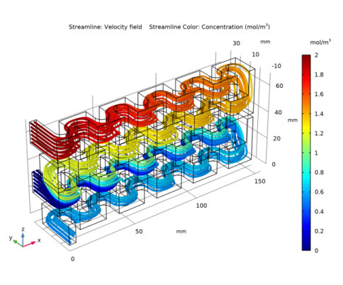
Figure 2 shows the streamlines of the fluid flow in the reactor plate. The color scale indicates the concentration of reactant A.
Figure 2: Streamlines of the fluid flow with the concentration of reactant A indicated by the color scale.
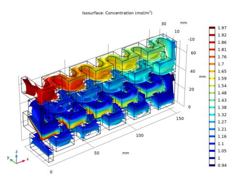
The isosurfaces for the concentration of reactant B are shown in Figure 3. The chemical reactions clearly consume the reactant along the entire reactor volume. The injection stream at the second inlet port mixes with the main stream, in effect making the distribution of B more uniform in the second part of the reactor.
Figure 3: The concentration of reactant B (mol/m3) across the reactor volume.
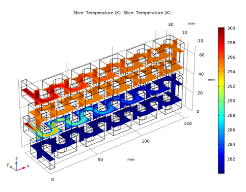
Figure 4 shows the temperature distribution, represented by horizontal and vertical cut planes.
Figure 4: Temperature distribution in the reactor plate.
Heat expelled by the reactions is seen to be quenched by the cooling in all parts of the reactor.
Application Library path: Chemical_Reaction_Engineering_Module/Reactors_with_Mass_and_Heat_Transfer/plate_reactor
Modeling Instructions
From the File menu, choose New.
New
In the New window, click  Model Wizard.
Model Wizard
1
In the Model Wizard window, click  3D.
2
In the Select Physics tree, select Fluid Flow>Single-Phase Flow>Laminar Flow (spf).
3
Click Add.
4
In the Select Physics tree, select Chemical Species Transport>Chemistry (chem).
5
Click Add.
6
In the Select Physics tree, select Heat Transfer>Heat Transfer in Fluids (ht).
7
Click Add.
8
In the Select Physics tree, select Chemical Species Transport>Transport of Diluted Species (tds).
9
Click Add.
10
In the Number of species text field, type 4.
11
In the Concentrations table, enter the following settings:
12
Click  Study.
13
In the Select Study tree, select General Studies>Stationary.
14
Geometry 1
Insert the geometry sequence.
1
In the Geometry toolbar, click  Insert Sequence.
2
3
In the Geometry toolbar, click  Build All.
Global Definitions
Load the model parameters from a text file.
Parameters 1
1
In the Model Builder window, under Global Definitions click Parameters 1.
2
In the Settings window for Parameters, locate the Parameters section.
3
Click  Load from File.
4
Definitions
Variables 1
1
In the Home toolbar, click  Variables and choose Local Variables.
2
In the Settings window for Variables, locate the Variables section.
3
Add Material
1
In the Home toolbar, click  Add Material to open the Add Material window.
2
Go to the Add Material window.
3
In the tree, select Liquids and Gases>Liquids>Water.
4
Click Add to Component in the window toolbar.
5
In the Home toolbar, click  Add Material to close the Add Material window.
Laminar Flow (spf)
1
In the Model Builder window, under Component 1 (comp1) click Laminar Flow (spf).
2
In the Settings window for Laminar Flow, locate the Physical Model section.
3
From the Compressibility list, choose Weakly compressible flow.
Inlet 1
1
In the Physics toolbar, click  Boundaries and choose Inlet.
2
In the Settings window for Inlet, locate the Boundary Selection section.
3
From the Selection list, choose Inlet 1.
4
Locate the Boundary Condition section. From the list, choose Fully developed flow.
5
Locate the Fully Developed Flow section. In the Uav text field, type U1.
Inlet 2
1
In the Physics toolbar, click  Boundaries and choose Inlet.
2
In the Settings window for Inlet, locate the Boundary Selection section.
3
From the Selection list, choose Inlet 2.
4
Locate the Boundary Condition section. From the list, choose Fully developed flow.
5
Locate the Fully Developed Flow section. In the Uav text field, type U2.
Chemistry (chem)
1
In the Model Builder window, under Component 1 (comp1) click Chemistry (chem).
2
In the Settings window for Chemistry, locate the Model Input section.
3
From the T list, choose Temperature (ht).
Reaction 1
1
In the Physics toolbar, click  Domains and choose Reaction.
2
In the Settings window for Reaction, locate the Reaction Formula section.
3
In the Formula text field, type A+B=>D.
4
Click Apply.
5
Locate the Rate Constants section. Select the Use Arrhenius expressions check box.
6
In the Af text field, type Af1.
7
In the Ef text field, type Ef1.
8
Locate the Reaction Thermodynamic Properties section. From the Enthalpy of reaction list, choose User defined.
9
In the H text field, type H1.
Reaction 2
1
In the Physics toolbar, click  Domains and choose Reaction.
2
In the Settings window for Reaction, locate the Reaction Formula section.
3
In the Formula text field, type D+B=>U.
4
Click Apply.
5
Locate the Rate Constants section. Select the Use Arrhenius expressions check box.
6
In the Af text field, type Af2.
7
In the Ef text field, type Ef2.
8
Locate the Reaction Thermodynamic Properties section. From the Enthalpy of reaction list, choose User defined.
9
In the H text field, type H2.
Species 1
1
In the Physics toolbar, click  Domains and choose Species.
2
In the Settings window for Species, locate the Species Name section.
3
4
In the Model Builder window, click Chemistry (chem).
5
In the Settings window for Chemistry, locate the Species Matching section.
6
Find the Bulk species subsection. In the table, enter the following settings:
7
Click to expand the Mixture Properties section. From the Phase list, choose Liquid.
Species: A
1
In the Model Builder window, click Species: A.
2
In the Settings window for Species, locate the General Parameters section.
3
In the M text field, type Mn_A.
Species: B
1
In the Model Builder window, click Species: B.
2
In the Settings window for Species, locate the General Parameters section.
3
In the M text field, type Mn_B.
Species: D
1
In the Model Builder window, click Species: D.
2
In the Settings window for Species, locate the General Parameters section.
3
In the M text field, type Mn_D.
Species: U
1
In the Model Builder window, click Species: U.
2
In the Settings window for Species, locate the General Parameters section.
3
In the M text field, type Mn_U.
Species: H2O
1
In the Model Builder window, click Species: H2O.
2
In the Settings window for Species, locate the General Parameters section.
3
In the M text field, type Mn_solv.
Laminar Flow (spf)
In the Model Builder window, under Component 1 (comp1) click Laminar Flow (spf).
Outlet 1
1
In the Physics toolbar, click  Boundaries and choose Outlet.
2
In the Settings window for Outlet, locate the Boundary Selection section.
3
From the Selection list, choose Outlet.
Activate normal flow to model that the channel is continuous after the outlet.
4
Locate the Pressure Conditions section. Select the Normal flow check box.
Heat Transfer in Fluids (ht)
Initial Values 1
1
In the Model Builder window, under Component 1 (comp1)>Heat Transfer in Fluids (ht) click Initial Values 1.
2
In the Settings window for Initial Values, locate the Initial Values section.
3
In the T text field, type T0.
Heat Source 1
1
In the Physics toolbar, click  Domains and choose Heat Source.
2
In the Settings window for Heat Source, locate the Heat Source section.
3
From the Q0 list, choose Heat source of reactions (chem).
4
Locate the Domain Selection section. From the Selection list, choose All domains.
Temperature 1
1
In the Physics toolbar, click  Boundaries and choose Temperature.
2
In the Settings window for Temperature, locate the Boundary Selection section.
3
From the Selection list, choose Inlet 1.
4
Locate the Temperature section. In the T0 text field, type T0.
Temperature 2
1
In the Physics toolbar, click  Boundaries and choose Temperature.
2
In the Settings window for Temperature, locate the Boundary Selection section.
3
From the Selection list, choose Inlet 2.
4
Locate the Temperature section. In the T0 text field, type T0.
Outflow 1
1
In the Physics toolbar, click  Boundaries and choose Outflow.
2
In the Settings window for Outflow, locate the Boundary Selection section.
3
From the Selection list, choose Outlet.
Heat Flux 1
1
In the Physics toolbar, click  Boundaries and choose Heat Flux.
2
In the Settings window for Heat Flux, locate the Boundary Selection section.
3
From the Selection list, choose Heat Exchanger 1.
4
Locate the Heat Flux section. In the q0 text field, type Q_exch1.
Heat Flux 2
1
In the Physics toolbar, click  Boundaries and choose Heat Flux.
2
In the Settings window for Heat Flux, locate the Boundary Selection section.
3
From the Selection list, choose Heat Exchanger 2.
4
Locate the Heat Flux section. In the q0 text field, type Q_exch2.
Transport of Diluted Species (tds)
Transport Properties 1
1
In the Model Builder window, under Component 1 (comp1)>Transport of Diluted Species (tds) click Transport Properties 1.
2
In the Settings window for Transport Properties, locate the Diffusion section.
3
In the DcA text field, type D.
4
In the DcB text field, type D.
5
In the DcD text field, type D.
6
In the DcU text field, type D.
Reactions 1
1
In the Physics toolbar, click  Domains and choose Reactions.
2
In the Settings window for Reactions, locate the Domain Selection section.
3
From the Selection list, choose All domains.
4
Locate the Reaction Rates section. From the RcA list, choose Reaction rate for species A (chem).
5
From the RcB list, choose Reaction rate for species B (chem).
6
From the RcD list, choose Reaction rate for species D (chem).
7
From the RcU list, choose Reaction rate for species U (chem).
Inflow 1
1
In the Physics toolbar, click  Boundaries and choose Inflow.
2
In the Settings window for Inflow, locate the Boundary Selection section.
3
From the Selection list, choose Inlet 1.
4
Locate the Concentration section. In the c0,cA text field, type cA1.
5
In the c0,cB text field, type cB1.
Inflow 2
1
In the Physics toolbar, click  Boundaries and choose Inflow.
2
In the Settings window for Inflow, locate the Boundary Selection section.
3
From the Selection list, choose Inlet 2.
4
Locate the Concentration section. In the c0,cB text field, type cB2.
Outflow 1
1
In the Physics toolbar, click  Boundaries and choose Outflow.
2
In the Settings window for Outflow, locate the Boundary Selection section.
3
From the Selection list, choose Outlet.
Multiphysics
Couple all interfaces except the Chemistry node with the Multiphysics node.
Nonisothermal Flow 1 (nitf1)
In the Physics toolbar, click  Multiphysics Couplings and choose Domain>Nonisothermal Flow.
Reacting Flow, Diluted Species 1 (rfd1)
In the Physics toolbar, click  Multiphysics Couplings and choose Domain>Reacting Flow, Diluted Species.
Mesh 1
Free Triangular 1
1
In the Mesh toolbar, click  Boundary and choose Free Triangular.
2
Size
1
In the Model Builder window, click Size.
2
In the Settings window for Size, locate the Element Size section.
3
Click the Custom button.
4
Locate the Element Size Parameters section. In the Maximum element size text field, type 1.
5
In the Minimum element size text field, type 0.5.
6
In the Resolution of narrow regions text field, type 0.2.
Swept 1
1
In the Mesh toolbar, click  Swept.
2
In the Settings window for Swept, locate the Domain Selection section.
3
From the Geometric entity level list, choose Domain.
4
5
Click  Build Selected.
Free Triangular 2
1
In the Model Builder window, under Component 1 (comp1)>Mesh 1 right-click Free Triangular 1 and choose Duplicate.
2
In the Settings window for Free Triangular, locate the Boundary Selection section.
3
Click  Clear Selection.
4
5
Click  Build Selected.
Swept 2
1
In the Mesh toolbar, click  Swept.
2
In the Settings window for Swept, click  Build All.
Study 1
Stationary 2
In the Study toolbar, click  Study Steps and choose Stationary>Stationary.
Stationary 3
In the Study toolbar, click  Study Steps and choose Stationary>Stationary.
Step 1: Stationary
1
In the Model Builder window, click Step 1: Stationary.
2
In the Settings window for Stationary, locate the Physics and Variables Selection section.
3
In the table, clear the Solve for check boxes for Chemistry (chem), Heat Transfer in Fluids (ht), and Transport of Diluted Species (tds).
Step 2: Stationary 2
1
In the Model Builder window, click Step 2: Stationary 2.
2
In the Settings window for Stationary, locate the Physics and Variables Selection section.
3
In the table, clear the Solve for check boxes for Laminar Flow (spf) and Heat Transfer in Fluids (ht).
Step 3: Stationary 3
1
In the Model Builder window, click Step 3: Stationary 3.
2
In the Settings window for Stationary, locate the Physics and Variables Selection section.
3
In the table, clear the Solve for check boxes for Laminar Flow (spf) and Transport of Diluted Species (tds).
4
In the Study toolbar, click  Compute.
Results
Velocity field
1
In the Home toolbar, click  Add Plot Group and choose 3D Plot Group.
2
In the Settings window for 3D Plot Group, type Velocity field in the Label text field.
3
Locate the Color Legend section. Select the Show units check box.
Streamline 1
1
Right-click Velocity field and choose Streamline.
2
3
In the Settings window for Streamline, locate the Coloring and Style section.
4
Find the Line style subsection. From the Type list, choose Tube.
5
In the Tube radius expression text field, type 5e-4.
6
Click the  Go to Default View button in the Graphics toolbar.
Color Expression 1
1
Right-click Streamline 1 and choose Color Expression.
2
In the Settings window for Color Expression, click Replace Expression in the upper-right corner of the Expression section. From the menu, choose Component 1 (comp1)>Transport of Diluted Species>Species cA>cA - Concentration - mol/m³.
3
Click to expand the Title section. From the Title type list, choose Automatic.
4
In the Velocity field toolbar, click  Plot.
5
Click the  Zoom Extents button in the Graphics toolbar.
3D Plot Group 14
In the Home toolbar, click  Add Plot Group and choose 3D Plot Group.
Slice 1
1
Right-click 3D Plot Group 14 and choose Slice.
2
In the Settings window for Slice, click Replace Expression in the upper-right corner of the Expression section. From the menu, choose Component 1 (comp1)>Heat Transfer in Fluids>Temperature>T - Temperature - K.
3
Locate the Plane Data section. From the Plane list, choose xy-planes.
4
In the Planes text field, type 4.
Temperature
1
In the Model Builder window, under Results click 3D Plot Group 14.
2
In the Settings window for 3D Plot Group, type Temperature in the Label text field.
Slice 2
1
Right-click Temperature and choose Slice.
2
In the Settings window for Slice, click Replace Expression in the upper-right corner of the Expression section. From the menu, choose Component 1 (comp1)>Heat Transfer in Fluids>Temperature>T - Temperature - K.
3
Locate the Plane Data section. From the Plane list, choose zx-planes.
4
In the Planes text field, type 1.
As you can see, the two color legends are nearly aligned so a single legend is sufficient.
5
Locate the Coloring and Style section. Clear the Color legend check box.
6
In the Temperature toolbar, click  Plot.
7
Click the  Zoom Extents button in the Graphics toolbar.
Concentration B
1
In the Home toolbar, click  Add Plot Group and choose 3D Plot Group.
2
In the Settings window for 3D Plot Group, type Concentration B in the Label text field.
Isosurface 1
1
Right-click Concentration B and choose Isosurface.
2
In the Settings window for Isosurface, click Replace Expression in the upper-right corner of the Expression section. From the menu, choose Component 1 (comp1)>Transport of Diluted Species>Species cB>cB - Concentration - mol/m³.
3
Locate the Levels section. In the Total levels text field, type 20.
4
In the Concentration B toolbar, click  Plot.
5
Click the  Zoom Extents button in the Graphics toolbar.