Parameter Estimation for Nonideal Reactor Models

You are viewing the documentation for an older COMSOL version. The latest version is available here.

PDF

Parameter Estimation for Nonideal Reactor Models

Real reactors can be modeled as combinations of ideal reactors. In this example, the “Dead zone model” is utilized. Two ideal CSTRs with interchange are used to model a real reactor. One CSTR represents the highly agitated region and the other one the less agitated region. Two parameters relating the volume and exchange rate of the two regions are required for this. The parameters are found by comparing the model results to experimental tracer data. Applying the Parameter Estimation feature in the Reaction Engineering interface makes this an easy task.

A problem description similar to the model presented here is given in Ref. 1.

This application requires the Optimization Module and the Chemical Reaction Engineering Module.

Model Definition

Two ideal CSTRs with interchange capture the essential behavior of a real reactor system.

Figure 1: A real reactor can be modeled by two ideal CSTRs with interchange.

The highly agitated volume is represented by V1 and the less agitated region by V2. The total real reactor volume is defined as:

(1)

and the parameter α gives the fraction of the total volume that belongs to V1:

Fluid is exchanged between volumes at a rate of v1 (SI unit: m3/s), and the parameter β relates this rate to the inlet flow rate:

Assuming that the reactor volume is constant, then the space time, τ (SI unit: s), is:

To evaluate the parameters α and β, a tracer compound is added through the reactor inlet stream, after which a response curve is measured at the outlet. Mass balances over the two CSTRs provide a model to which the experimental data can be compared. The mass balances are:

where cT1 is the tracer concentration (SI unit: mol /m3) in the region given by V1, and cT2 is the tracer concentration in V2. cT0 is the tracer amount into the real reactor. The tracer compound is said to be diluted in water.

This coupled set of ODEs can easily be set up by combining two Reaction Engineering interfaces where the reactor type is set to .

Experimental data

An experiment is performed where a 1000 mol/m3 tracer solution is added in the reactor feed inlet stream. The tracer concentration in the reactor outlet stream is then recorded as a function of time. The data is presented in Table 1 below.

Table 1: Experimental data.
Time (s)	Concentration (mol/m3)
600	242
1200	446
1800	585
2400	668
3600	795
6000	909
9000	953
18000	991
24000	994

The Parameter Estimation feature accepts comma-separated value files (csv-files) for import of experimental data into the software. After import, the columns of the data file are shown and are mapped to the model variables.

Results and Discussion

Figure 2 shows the model results, both when using an initial guess, and when using parameter estimation. The figure also shows the experimental data. The results from the parameter estimation are seen to coincide well with the experimental data.

Figure 2: Model results and experimental data of the tracer concentration in the real reactor outlet.

The estimated values of α and β are 0.83 and 0.11, respectively.

1. H.S. Fogler, Elements in Chemical Reaction Engineering, 4th ed., Prentice Hall, pp. 985–987, 2005.

Chemical_Reaction_Engineering_Module/Tutorials/nonideal_cstr

Modeling Instructions

From the menu, choose .

In the window, click

.

1

In the window, click

.

2

In the tree, select .

3

4

5

In the tree, select .

6

Global Definitions

Add a set of model parameters by importing their definitions from a data text file provided with the .

1

In the window, under click .

2

In the window for , locate the section.

3

.

4

Browse to the model’s Application Libraries folder and double-click the file nonideal_cstr_parameters.txt.

Start defining the first CSTR representing the highly agitated zone.

Reaction Engineering - CSTR 1

1

In the window, under click .

2

In the window for , type Reaction Engineering - CSTR 1 in the text field.

3

In the text field, type re1.

4

Locate the section. From the list, choose .

5

Locate the section. From the list, choose .

6

Locate the section. Find the subsection. From the list, choose .

Two streams are assumed to exit the first CSTR: v0 and v0*beta.

7

In the v text field, type (1+beta)*v0.

1

In the toolbar, click

.

2

In the window for , locate the section.

3

In the text field, type T.

4

In the toolbar, click

.

1

In the window for , locate the section.

2

In the text field, type H2O.

3

Locate the section. From the list, choose .

1

In the window, click .

2

In the window for , locate the section.

3

In the M text field, type Mn_T.

1

In the window, click .

2

In the window for , locate the section.

3

In the M text field, type Mn_w.

4

In the ρ text field, type rho_w.

Initial Values 1

The first CSTR has an initial volume alpha times the total real reactor volume.

1

In the window, click .

2

In the window for , locate the section.

3

In the Vr0 text field, type alpha*Vtot.

4

Locate the section. In the table, enter the following settings:


Species	Concentration (mol/m^3)
H2O	c_w

Add two feed inlet streams to the first CSTR. One representing the flow entering the real reactor, v0, and another one representing the stream from the second CSTR, v0*beta.

1

In the toolbar, click

.

2

In the window for , locate the section.

3

In the vf text field, type v0.

4

Locate the section. In the table, enter the following settings:


Species	Concentration (mol/m^3)
H2O	c_w
T	c_T0

1

In the toolbar, click

.

2

In the window for , locate the section.

3

In the vf text field, type v0*beta.

4

Locate the section. In the table, enter the following settings:


Species	Concentration (mol/m^3)
H2O	c_w
T	re2.c_T

Continue to define the second CSTR representing the dead zone. To do this copy the first interface.

5

In the window, right-click and choose .

Reaction Engineering - CSTR 2

1

In the window, right-click and choose .

2

In the dialog box, click .

3

In the window for , type Reaction Engineering - CSTR 2 in the text field.

Only one stream exits the second CSTR: v0*beta.

4

Locate the section. Find the subsection. In the v text field, type v0*beta.

Initial Values 1

The second CSTR has an initial volume (1-alpha) times the total real reactor volume.

1

In the window, expand the node, then click .

2

In the window for , locate the section.

3

In the Vr0 text field, type (1-alpha)*Vtot.

4

Locate the section. In the table, enter the following settings:


Species	Concentration (mol/m^3)
H2O	c_w

1

In the window, click .

2

In the window for , locate the section.

3

In the vf text field, type v0*beta.

4

Locate the section. In the table, enter the following settings:


Species	Concentration (mol/m^3)
T	re1.c_T

Remove the second feed inlet stream.

In the window, right-click and choose .

Reaction Engineering - CSTR 1 (re1)

Now add a feature to be used in the optimization.

1

In the window, under click .

Parameter Estimation 1

1

In the toolbar, click

.

2

In the window for , locate the section.

3

In the table, enter the following settings:


Parameter	Initial value	Scale	Lower bound	Upper bound
alpha	0.5	1

4

5

In the table, enter the following settings:


Parameter	Initial value	Scale	Lower bound	Upper bound
beta	0.1	1

1

In the toolbar, click

and choose .

Read in the csv-file with the and map the data columns with the model variables.

2

In the window for , locate the section.

3

4

Browse to the model’s Application Libraries folder and double-click the file nonideal_cstr_data.csv.

5

6

In the table, enter the following settings:


Data column	Use	Model variables	Unit	Weight
Tracer (mol/m3)	√	c_T	1	1

Solve the model using the initial values of the alpha and beta parameters.

Study 1: Initial guess

1

In the window, click .

2

In the window for , type Study 1: Initial guess in the text field.

Step 1: Time Dependent

1

In the window, under click .

2

In the window for , locate the section.

3

In the text field, type 24000.

Disable the feature for this study step.

4

Locate the section. Select the check box.

5

In the tree, select .

6

7

In the toolbar, click

.

The following instructions generate Figure 2.

Concentration in Real Reactor

1

In the window, under click .

2

In the window for , type Concentration in Real Reactor in the text field.

3

Click to expand the section. From the list, choose .

4

Locate the section. Select the check box.

5

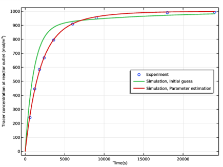
In the associated text field, type Time(s).

6

Select the check box.

7

In the associated text field, type Tracer concentration at reactor outlet (mol/m<sup>3</sup>).

8

Locate the section. From the list, choose .

1

In the window, expand the node, then click .

2

In the window for , type Experiment in the text field.

3

Click to expand the section. From the list, choose .

4

In the table, enter the following settings:


Legends
Experiment

Simulation, Initial guess

1

In the window, right-click and choose .

2

In the window for , locate the section.

3

From the list, choose .

4

Locate the section. In the table, enter the following settings:


Expression	Unit	Description

5

In the text field, type Simulation, Initial guess.

6

Click to expand the section. In the text field, type 2.

7

Click to expand the section. From the list, choose .

8

In the table, enter the following settings:


Legends
Simulation, Initial guess

9

In the toolbar, click

.

The following instructions generate a figure with tracer concentrations in the two CSTRs.

Concentrations in CSTRs

1

In the window, under click .

2

In the window for , type Concentrations in CSTRs in the text field.

3

Locate the section. Select the check box.

4

In the associated text field, type Tracer concentrations (mol/m<sup>3</sup>).

5

Locate the section. From the list, choose .

1

In the window, expand the node, then click .

2

In the window for , click in the upper-right corner of the section. From the menu, choose .

3

Locate the section. In the text field, type 2.

4

Locate the section. From the list, choose .

5

In the table, enter the following settings:


Legends
Ideal tank 1
Ideal tank 2

6

In the toolbar, click

.

The third plot group will not be used and can be deleted.

Concentration (re2)

In the window, right-click and choose .

Add a new study node for the optimization calculations.

1

In the toolbar, click

to open the window.

2

Go to the window.

3

Find the subsection. In the tree, select .

4

Click in the window toolbar.

5

In the toolbar, click

to close the window.

Step 1: Time Dependent

1

In the window for , locate the section.

2

In the text field, type 24000.

Add an study step to perform the parameter estimation calculations.

3

In the window, click .

4

In the window for , type Study 2: Parameter estimation in the text field.

1

In the toolbar, click

.

Select to use the Levenberg-Marquardt optimization method. This method is very efficient for this type of optimization; when no mesh is effected and no additional constraints are present.

2

In the window for , locate the section.

3

From the list, choose .

The existing plots will be reused. Disable the generation of default plots.

4

In the window, click .

5

In the window for , locate the section.

6

Clear the check box.

Solution 2 (sol2)

1

In the toolbar, click

.

2

In the window for , click

.

Simulation, Parameter estimation

1

In the window, right-click and choose .

2

In the window for , type Simulation, Parameter estimation in the text field.

3

Locate the section. From the list, choose .

4

Locate the section. In the table, enter the following settings:


Legends
Simulation, Parameter estimation

5

In the toolbar, click

.

Concentrations in CSTRs

1

In the window, click .

2

In the window for , locate the section.

3

From the list, choose .

4

In the toolbar, click

.

Display the estimated parameters in a table.

Global Evaluation 1

1

In the toolbar, click

.

2

In the window for , locate the section.

3

From the list, choose .

4

From the list, choose .

5

Click in the upper-right corner of the section. From the menu, choose .

6

Click in the upper-right corner of the section. From the menu, choose .

7