PDF

Laminar Static Mixer
Introduction
In static mixers, also called motionless or in-line mixers, a fluid is pumped through a pipe containing stationary blades. This mixing technique is particularly well suited for laminar flow mixing because it generates only small pressure losses in this flow regime. This example studies the flow in a twisted-blade static mixer.
Model Definition
This model studies the mixing of one species dissolved in water at room temperature. The geometry consists of a tube with three twisted blades of alternating rotations (Figure 1).
Figure 1: Depiction of a laminar static mixer containing three blades with alternating rotations.
The tube’s radius, R, is 3 mm; the length is 14R, and the length of each blade is 3R. The inlet flow is laminar with an average velocity of 10 mm/s. At the outlet, the model specifies a constant reference pressure of 0 Pa. The Laminar Flow interface is used in 3D and solves the Navier-Stokes equations:
(1)
Here μ denotes the dynamic viscosity (SI unit: kg/(m·s)), u is the velocity (SI unit: m/s), ρ represents the fluid density (SI unit: kg/m3), and p denotes the pressure (SI unit: Pa). These fluid flow properties are not affected by any change in concentration of the dissolved species and are imported from the Material Library.
The species transport, which is defined in the Transport of Diluted Species interface, consists of convection and diffusion. At the outlet an Outflow boundary node is used to prescribe vanishing diffusion in the normal direction. At the inlet, a step change of the concentration is applied using an Inlet node. The inlet concentration is defined as:
(2)
The concentration changes smoothly across a small transition zone δ = 0.3 mm. Due to the sharp concentration gradient and the fact that the convection is included, a fine mesh is required in order to avoid oscillations in the concentration field. The Reynolds numbers in the mixer, based on the average velocity and the diameter of the pipe, is about 60. This indicates that the flow is laminar and the fluid flow (Equation 1) does not require a particularly dense mesh near the walls. The Peclet number for the mass transport on the other hand is significantly higher.
This means that the concentration gradient will be thinner than the shear layers in the flow. Consequently a higher resolution is needed for the mass transport compared to that for fluid flow. Since the concentration does not influence the fluid flow, you can therefore first solve the Navier-Stokes equations on a coarse mesh, and then map the solution onto a finer mesh and solve for the mass transport. In this model the resolution is further increased by using second order elements for the species concentration.
Results
Figure 2 shows a slice plot of the concentration in the mixer. The slice at the bottom shows the blue and red halves of the fluid with and without the dissolved species, respectively. As the fluid flows upward through the system, the two solutions are mixed producing a more homogeneous concentration profile at the outlet.
Figure 2: Slice plot of the concentration at different distances from the inlet.
Figure 3 shows the flow field responsible for the mixing. The streamlines clearly reveal the twisting motion in the fluid that is induced by the mixer blades.
Figure 3: Slice plots of the velocity magnitude field inside the mixer. The streamlines show the flow direction.
You can also visualize the mixing through a series of cross-section plots. Figure 4 contains such a series of plots showing the concentration in the mixer’s cross section along the direction of the flow. The results show that most of the mixing takes place where the blades change rotational direction (the three middle figures).
Figure 4: Cross-sectional plots of the concentration at different distances from the inlet. The nine plots shows the concentration at z =- 2 mm to z = 30 mm in steps of 4 mm.
References
1. R. Perry and D. Green, Perry’s Chemical Engineering Handbook, 7th ed., McGraw-Hill, 1997.
2. J.M. Coulson and J.F. Richardson, Chemical Engineering, vol. 1, 4th ed., Pergamon Press, 1990.
Application Library path: Chemical_Reaction_Engineering_Module/Mixing_and_Separation/laminar_static_mixer
Modeling Instructions
From the File menu, choose New.
New
In the New window, click  Model Wizard.
Model Wizard
1
In the Model Wizard window, click  3D.
2
In the Select Physics tree, select Fluid Flow>Single-Phase Flow>Laminar Flow (spf).
3
Click Add.
4
In the Select Physics tree, select Chemical Species Transport>Transport of Diluted Species (tds).
5
Click Add.
6
Click  Study.
7
In the Select Study tree, select General Studies>Stationary.
8
Geometry 1
Import the model parameters from a text file.
Global Definitions
Parameters 1
1
In the Model Builder window, under Global Definitions click Parameters 1.
2
In the Settings window for Parameters, locate the Parameters section.
3
Click  Load from File.
4
A Step function is required to create a step change in the concentration at the inlet of the mixer.
Step 1 (step1)
1
In the Home toolbar, click  Functions and choose Global>Step.
2
In the Settings window for Step, locate the Parameters section.
3
In the To text field, type 5.
4
Click to expand the Smoothing section. In the Size of transition zone text field, type 3e-4.
Create the geometry. To simplify this step, insert a prepared geometry sequence. In the Geometry toolbar, click Insert Sequence. Browse to the model’s Application Libraries folder and double-click the file laminar_static_mixer.mph. Then click Build All In the Geometry toolbar.
Add Material
1
In the Home toolbar, click  Add Material to open the Add Material window.
2
Go to the Add Material window.
3
In the tree, select Built-in>Water, liquid.
4
Click Add to Component in the window toolbar.
5
In the Home toolbar, click  Add Material to close the Add Material window.
Materials
Water, liquid (mat1)
The first material you add applies to all domains by default, so you do not need to change any settings.
In the Laminar Flow interface, set Inlet and outlet boundary conditions together with the initial values.
Laminar Flow (spf)
Inlet 1
1
In the Model Builder window, under Component 1 (comp1) right-click Laminar Flow (spf) and choose Inlet.
2
3
In the Settings window for Inlet, locate the Boundary Condition section.
4
From the list, choose Fully developed flow.
5
Locate the Fully Developed Flow section. In the Uav text field, type u_av.
This gives a parabolic inlet velocity profile, appropriate for fully developed laminar flow, with mean velocity u_av.
Outlet 1
1
In the Physics toolbar, click  Boundaries and choose Outlet.
2
Apply quadratic basis functions for the concentration to further increase the resolution.
Transport of Diluted Species (tds)
1
In the Model Builder window, under Component 1 (comp1) click Transport of Diluted Species (tds).
2
In the Settings window for Transport of Diluted Species, click to expand the Discretization section.
3
From the Concentration list, choose Quadratic.
In the Transport of Diluted interface, apply inlet and outlet boundary conditions together with initial values. The velocity from the Laminar Flow interface is automatically applied for the convective transport by the Reacting Flow, Diluted Species Multiphysics feature.
Transport Properties 1
1
In the Model Builder window, under Component 1 (comp1)>Transport of Diluted Species (tds) click Transport Properties 1.
2
In the Settings window for Transport Properties, locate the Diffusion section.
3
In the Dc text field, type D.
Inflow 1
1
In the Physics toolbar, click  Boundaries and choose Inflow.
At the inlet use the Step function to introduce a sharp but continuous step in the concentration.
2
In the Settings window for Inflow, locate the Concentration section.
3
In the c0,c text field, type step1(x[1/mm]).
4
Outflow 1
1
In the Physics toolbar, click  Boundaries and choose Outflow.
2
The Outflow feature assumes that the flow through the outlet is governed by the convection.
Multiphysics
Reacting Flow, Diluted Species 1 (rfd1)
In the Physics toolbar, click  Multiphysics Couplings and choose Domain>Reacting Flow, Diluted Species.
Two meshes are required: A course one for the Laminar Flow interface and a finer one for the Transport of Diluted Species interface.
Mesh 1
1
In the Model Builder window, under Component 1 (comp1) click Mesh 1.
2
In the Settings window for Mesh, locate the Physics-Controlled Mesh section.
3
From the Element size list, choose Extra coarse.
4
Click  Build All.
Mesh 2
In the Mesh toolbar, click  Add Mesh.
Free Tetrahedral 1
In the Mesh toolbar, click  Free Tetrahedral.
Size
1
In the Settings window for Size, locate the Element Size section.
2
Click the Custom button.
3
Locate the Element Size Parameters section. In the Maximum element size text field, type 0.65.
4
In the Minimum element size text field, type 0.35.
5
Click  Build All.
The study needs to be solved in two Stationary steps. First, the Laminar Flow is computed with Mesh 1. Second, the Transport of Diluted Species is calculated using Mesh 2.
Study 1
Stationary 2
In the Study toolbar, click  Study Steps and choose Stationary>Stationary.
Step 1: Stationary
1
In the Model Builder window, click Step 1: Stationary.
2
In the Settings window for Stationary, locate the Physics and Variables Selection section.
3
In the table, clear the Solve for check box for Transport of Diluted Species (tds).
Step 2: Stationary 2
1
In the Model Builder window, click Step 2: Stationary 2.
2
In the Settings window for Stationary, locate the Physics and Variables Selection section.
3
In the table, clear the Solve for check box for Laminar Flow (spf).
4
In the Study toolbar, click  Compute.
Results
To reproduce Figure 2, which uses a slice plot to visualize the concentration within the mixer, follow these steps.
Concentration, Slice
1
In the Home toolbar, click  Add Plot Group and choose 3D Plot Group.
2
In the Settings window for 3D Plot Group, type Concentration, Slice in the Label text field.
Slice 1
1
Right-click Concentration, Slice and choose Slice.
2
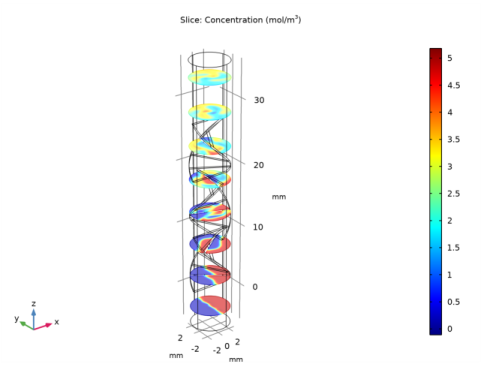
In the Settings window for Slice, click Replace Expression in the upper-right corner of the Expression section. From the menu, choose Component 1 (comp1)>Transport of Diluted Species>Species c>c - Concentration - mol/m³.
3
Locate the Plane Data section. From the Plane list, choose xy-planes.
4
In the Planes text field, type 8.
5
Click the  Zoom Extents button in the Graphics toolbar.
Since quadratic elements was applied for the concentration, the resolution of the plot can be increased.
6
Click to expand the Quality section. From the Resolution list, choose Finer.
7
In the Concentration, Slice toolbar, click  Plot.
Velocity (spf)
To create Figure 3 that displays the velocity field, follow these steps.
Streamline 1
1
In the Model Builder window, expand the Results>Velocity (spf) node.
2
Right-click Velocity (spf) and choose Streamline.
Slice
1
In the Settings window for Slice, locate the Plane Data section.
2
From the Plane list, choose xy-planes.
3
In the Planes text field, type 8.
Streamline 1
1
In the Model Builder window, click Streamline 1.
2
In the Settings window for Streamline, locate the Streamline Positioning section.
3
From the Positioning list, choose Magnitude controlled.
4
In the Min distance text field, type 0.025.
5
In the Max distance text field, type 0.1.
6
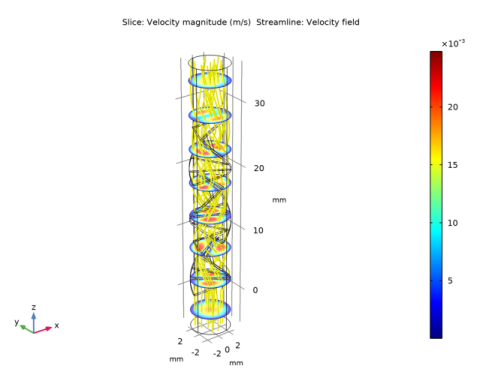
Locate the Coloring and Style section. Find the Line style subsection. From the Type list, choose Tube.
7
In the Tube radius expression text field, type 0.05.
8
Find the Point style subsection. From the Color list, choose Yellow.
9
Find the Line style subsection. Select the Radius scale factor check box.
10
11
In the Velocity (spf) toolbar, click  Plot.
Finally, reproduce the series of cross-sectional concentration plots for different z-coordinates shown in Figure 4 with the following steps.
Cut Plane 1
1
In the Results toolbar, click  Cut Plane.
2
In the Settings window for Cut Plane, locate the Plane Data section.
3
From the Plane list, choose xy-planes.
4
In the z-coordinate text field, type -2.
Cross-sectional concentration plot
1
In the Results toolbar, click  2D Plot Group.
2
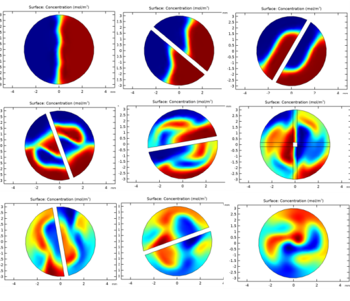
In the Settings window for 2D Plot Group, type Cross-sectional concentration plot in the Label text field.
3
Locate the Data section. From the Dataset list, choose Cut Plane 1.
Surface 1
1
Right-click Cross-sectional concentration plot and choose Surface.
2
In the Settings window for Surface, click Replace Expression in the upper-right corner of the Expression section. From the menu, choose Component 1 (comp1)>Transport of Diluted Species>Species c>c - Concentration - mol/m³.
3
Locate the Coloring and Style section. Clear the Color legend check box.
Increase the resolution also for this plot.
4
Click to expand the Quality section. From the Resolution list, choose Finer.
5
In the Cross-sectional concentration plot toolbar, click  Plot.
Cut Plane 1
1
In the Model Builder window, click Cut Plane 1.
2
In the Settings window for Cut Plane, locate the Plane Data section.
3
In the z-coordinate text field, type 2.
Cross-sectional concentration plot
Repeat these steps for z-coordinate 6, 10, 14, 18, 22, 26, and 30 to reproduce the remaining plots in Figure 4.
Cut Plane 1
1
In the Model Builder window, click Cut Plane 1.
2
In the Settings window for Cut Plane, locate the Plane Data section.
3
In the z-coordinate text field, type 6.
Cut Plane 1
1
In the Model Builder window, click Cut Plane 1.
2
In the Settings window for Cut Plane, locate the Plane Data section.
3
In the z-coordinate text field, type 10.
Cut Plane 1
1
In the Model Builder window, click Cut Plane 1.
2
In the Settings window for Cut Plane, locate the Plane Data section.
3
In the z-coordinate text field, type 14.
Cut Plane 1
1
In the Model Builder window, click Cut Plane 1.
2
In the Settings window for Cut Plane, locate the Plane Data section.
3
In the z-coordinate text field, type 18.
Cut Plane 1
1
In the Model Builder window, click Cut Plane 1.
2
In the Settings window for Cut Plane, locate the Plane Data section.
3
In the z-coordinate text field, type 22.
Cut Plane 1
1
In the Model Builder window, click Cut Plane 1.
2
In the Settings window for Cut Plane, locate the Plane Data section.
3
In the z-coordinate text field, type 26.
Cut Plane 1
1
In the Model Builder window, click Cut Plane 1.
2
In the Settings window for Cut Plane, locate the Plane Data section.
3
In the z-coordinate text field, type 30.