
|
|
|


|
1
|
|
2
|
|
3
|
Click Add.
|
|
4
|
Click
|
|
5
|
|
6
|
Click
|
|
1
|
|
2
|
|
3
|
|
4
|
Browse to the model’s Application Libraries folder and double-click the file hi_batch_reactor_parameters.txt.
|
|
1
|
|
2
|
|
3
|
|
4
|
|
1
|
|
2
|
|
3
|
|
4
|
|
5
|
|
6
|
|
7
|
|
8
|
|
1
|
|
2
|
|
1
|
In the Model Builder window, under Component 1 (comp1) right-click Definitions and choose Variables.
|
|
2
|
|
3
|
|
4
|
Browse to the model’s Application Libraries folder and double-click the file hi_batch_reactor_variables.txt.
|
|
5
|
|
1
|
|
2
|
Click Next in the window toolbar.
|
|
1
|
|
2
|
|
3
|
|
4
|
|
5
|
|
6
|
|
7
|
|
8
|
Click Next in the window toolbar.
|
|
1
|
|
2
|
Click Finish in the window toolbar.
|
|
1
|
|
2
|
|
3
|
Select the Thermodynamics check box.
|
|
4
|
|
5
|
|
1
|
|
2
|
|
3
|
|
4
|
|
1
|
|
2
|
|
1
|
|
2
|
|
3
|
Click OK.
|
|
1
|
|
2
|
|
3
|
From the list, choose Include.
|
|
1
|
In the Model Builder window, under Component 1 (comp1)>Reaction Engineering (re) click Initial Values 1.
|
|
2
|
|
3
|
|
1
|
|
2
|
|
3
|
Click OK.
|
|
1
|
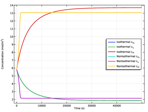
In the Model Builder window, expand the Results>Concentration (re) node, then click Concentration (re).
|
|
2
|
|
3
|
|
1
|
|
2
|
|
3
|
|
4
|
|
5
|
|
7
|
|
1
|
|
2
|
|
3
|
|
4
|
Locate the Legends section. In the table, enter the following settings:
|
|
5
|
|
1
|
|
2
|
|
3
|
|
4
|
Click OK.
|
|
5
|
|
6
|
|
7
|
|
8
|
In the associated text field, type Time (s).
|
|
9
|
|
10
|
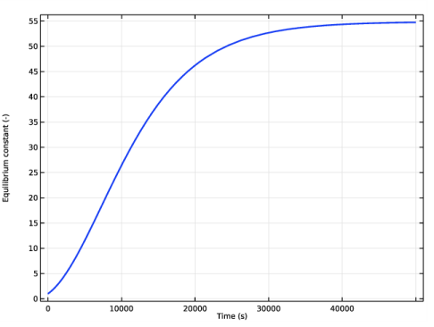
In the associated text field, type Equilibrium constant (-).
|
|
1
|
|
2
|
In the Settings window for Global, click Replace Expression in the upper-right corner of the y-Axis Data section. From the menu, choose Component 1 (comp1)>Definitions>Variables>K_equi - Equilibrium constant.
|
|
3
|
|
4
|
|
5
|
|
6
|
|
1
|
|
2
|
|
3
|
|
4
|
Click OK.
|
|
5
|
|
6
|
|
7
|
|
8
|
In the associated text field, type Time (s).
|
|
9
|
|
10
|
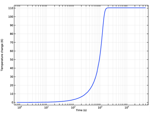
In the associated text field, type Temperature change (K).
|
|
11
|
|
1
|
|
2
|
In the Settings window for Global, click Replace Expression in the upper-right corner of the y-Axis Data section. From the menu, choose Component 1 (comp1)>Definitions>Variables>T_change - Temperature change - K.
|
|
3
|
|
4
|
|
5
|
|
6
|
|
1
|
|
2
|
|
3
|
|
1
|
|
2
|
|
3
|
|
4
|
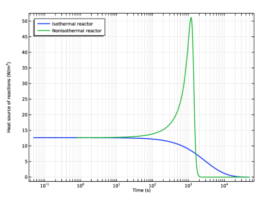
Click Add Expression in the upper-right corner of the y-Axis Data section. From the menu, choose Component 1 (comp1)>Reaction Engineering>re.Qheat - Heat source of reactions - W/m³.
|
|
5
|
|
6
|
|
8
|
|
9
|
|
1
|
|
2
|
|
4
|
|
1
|
|
2
|
|
3
|
|
4
|