|
|
|
|
3
|
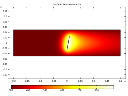
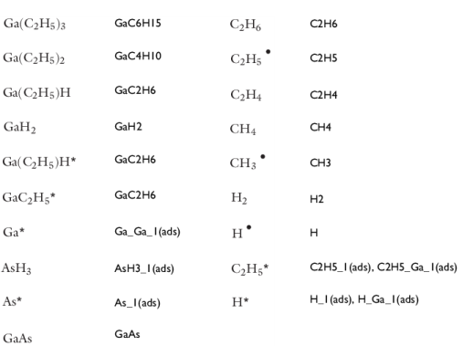
Growth of GaAs at the surface by the adsorption of gas phase species and the subsequent reaction of the surface-bonded molecular fragments. These surface reactions involve the Ga and As species. SA and SG represent surface sites, corresponding to dangling bonds of As or Ga atoms, respectively.
|


|
1
|
|
2
|
|
3
|
Click Add.
|
|
4
|
Click
|
|
5
|
|
6
|
Click
|
|
1
|
|
2
|
|
3
|
|
4
|
Browse to the model’s Application Libraries folder and double-click the file gaas_cvd_parameters.txt.
|
|
1
|
In the Model Builder window, under Component 1 (comp1) right-click Reaction Engineering (re) and choose Reversible Reaction Group.
|
|
2
|
In the Settings window for Reversible Reaction Group, click to expand the CHEMKIN Import for Kinetics section.
|
|
3
|
|
4
|
Click Browse.
|
|
5
|
Browse to the model’s Application Libraries folder and double-click the file gaas_cvd_reaction_kinetics.txt.
|
|
6
|
Click Import.
|
|
1
|
In the Model Builder window, expand the Component 1 (comp1)>Reaction Engineering (re)>Species Group 1 node, then click Reaction Engineering (re).
|
|
2
|
|
3
|
|
1
|
|
2
|
In the Settings window for Reversible Reaction Group, locate the CHEMKIN Import for Kinetics section.
|
|
3
|
|
4
|
Click to expand the Move Reaction and Species section. In the Move reaction (with the number) from table text field, type 9.
|
|
5
|
|
1
|
|
2
|
|
3
|
From the list, choose Solvent.
|
|
1
|
|
2
|
|
1
|
In the Model Builder window, expand the Concentrations full reaction set (re) node, then click Global 1.
|
|
2
|
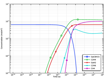
In the Settings window for Global, click Replace Expression in the upper-right corner of the y-Axis Data section. From the menu, choose Component 1 (comp1)>Reaction Engineering>re.c_GaC6H15 - Concentration - mol/m³.
|
|
3
|
Click Add Expression in the upper-right corner of the y-Axis Data section. From the menu, choose Component 1 (comp1)>Reaction Engineering>re.c_C2H4 - Concentration - mol/m³.
|
|
4
|
Click Add Expression in the upper-right corner of the y-Axis Data section. From the menu, choose Component 1 (comp1)>Reaction Engineering>re.c_GaH2 - Concentration - mol/m³.
|
|
5
|
Click Add Expression in the upper-right corner of the y-Axis Data section. From the menu, choose Component 1 (comp1)>Reaction Engineering>re.c_C2H6 - Concentration - mol/m³.
|
|
6
|
Click Add Expression in the upper-right corner of the y-Axis Data section. From the menu, choose Component 1 (comp1)>Reaction Engineering>re.c_CH4 - Concentration - mol/m³.
|
|
7
|
|
8
|
|
9
|
|
11
|
|
12
|
|
1
|
|
2
|
|
3
|
|
4
|
|
5
|
|
6
|
|
7
|
|
8
|
|
1
|
|
2
|
|
1
|
|
2
|
|
3
|
Click OK.
|
|
1
|
In the Model Builder window, expand the Component 1 (comp1)>Reaction Engineering (re)>Reversible Reaction Group 1 node, then click Results>Concentrations full reaction set (re).
|
|
2
|
|
3
|
|
1
|
In the Settings window for 1D Plot Group, type Concentrations reduced reaction set (re) in the Label text field.
|
|
1
|
In the Model Builder window, expand the Concentrations reduced reaction set (re) node, then click Global 1.
|
|
2
|
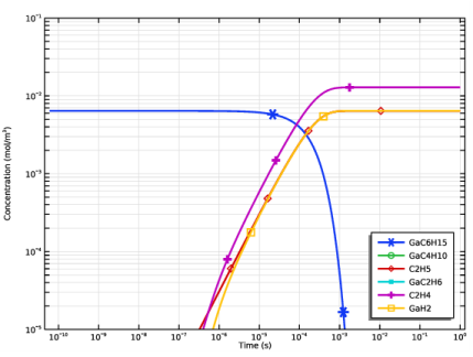
In the Settings window for Global, click Replace Expression in the upper-right corner of the y-Axis Data section. From the menu, choose Component 1 (comp1)>Reaction Engineering>re.c_GaC6H15 - Concentration - mol/m³.
|
|
3
|
Click Add Expression in the upper-right corner of the y-Axis Data section. From the menu, choose Component 1 (comp1)>Reaction Engineering>re.c_GaC4H10 - Concentration - mol/m³.
|
|
4
|
Click Add Expression in the upper-right corner of the y-Axis Data section. From the menu, choose Component 1 (comp1)>Reaction Engineering>re.c_C2H5 - Concentration - mol/m³.
|
|
5
|
Click Add Expression in the upper-right corner of the y-Axis Data section. From the menu, choose Component 1 (comp1)>Reaction Engineering>re.c_GaC2H6 - Concentration - mol/m³.
|
|
6
|
Click Add Expression in the upper-right corner of the y-Axis Data section. From the menu, choose Component 1 (comp1)>Reaction Engineering>re.c_C2H4 - Concentration - mol/m³.
|
|
7
|
Click Add Expression in the upper-right corner of the y-Axis Data section. From the menu, choose Component 1 (comp1)>Reaction Engineering>re.c_GaH2 - Concentration - mol/m³.
|
|
8
|
|
9
|
|
10
|
|
12
|
|
13
|
|
1
|
|
2
|
|
3
|
|
4
|
|
5
|
|
6
|
|
7
|
|
8
|
|
1
|
|
2
|
|
3
|
|
4
|
|
5
|
|
6
|
|
1
|
|
2
|
|
3
|
|
4
|
|
5
|
|
6
|
|
7
|
|
1
|
|
2
|
Select the object r1 only.
|
|
3
|
|
4
|
|
5
|
|
6
|
Select the object r2 only.
|
|
1
|
|
2
|
|
3
|
|
4
|
|
5
|
|
1
|
|
2
|
In the Settings window for Reversible Reaction Group, click to expand the CHEMKIN Import for Kinetics section.
|
|
3
|
|
4
|
Click Browse.
|
|
5
|
Browse to the model’s Application Libraries folder and double-click the file gaas_cvd_reaction_kinetics.txt.
|
|
6
|
Click Import.
|
|
7
|
|
8
|
|
1
|
|
2
|
|
3
|
Click Browse.
|
|
4
|
Browse to the model’s Application Libraries folder and double-click the file gaas_cvd_transp.txt.
|
|
5
|
Click Import.
|
|
1
|
|
2
|
In the Settings window for Species Thermodynamics, click to expand the CHEMKIN Import for Thermodynamic Data section.
|
|
3
|
Click Browse.
|
|
4
|
Browse to the model’s Application Libraries folder and double-click the file gaas_cvd_thermo.txt.
|
|
5
|
Click Import.
|
|
1
|
|
2
|
In the Settings window for Reversible Reaction Group, locate the CHEMKIN Import for Kinetics section.
|
|
3
|
|
4
|
Click to expand the Move Reaction and Species section. In the Move reaction (with the number) from table text field, type 9.
|
|
5
|
|
1
|
|
2
|
|
3
|
From the list, choose Solvent.
|
|
1
|
|
2
|
|
3
|
|
4
|
|
5
|
|
6
|
|
7
|
|
8
|
|
1
|
|
2
|
|
3
|
|
4
|
|
5
|
|
1
|
In the Settings window for Transport of Diluted Species, click to expand the Dependent Variables section.
|
|
2
|
|
3
|
In the Concentrations table, enter the following settings:
|
|
1
|
In the Model Builder window, expand the Component 2 (comp2)>Chemistry (chem) node, then click Component 2 (comp2)>Transport of Diluted Species (tds)>Transport Properties 1.
|
|
2
|
|
3
|
|
4
|
|
5
|
|
6
|
|
7
|
|
8
|
|
9
|
|
10
|
|
1
|
|
2
|
|
3
|
|
4
|
Locate the Reaction Rates section. From the RcGaC4H10 list, choose Reaction rate for species GaC4H10 (chem).
|
|
5
|
|
6
|
|
7
|
|
8
|
|
9
|
|
10
|
|
11
|
|
1
|
|
3
|
|
4
|
|
5
|
|
6
|
|
7
|
|
8
|
|
9
|
|
10
|
|
11
|
|
1
|
|
3
|
|
4
|
|
5
|
|
1
|
|
1
|
|
2
|
|
3
|
|
4
|
|
1
|
|
2
|
|
3
|
|
4
|
|
5
|
|
1
|
|
2
|
|
3
|
|
4
|
|
5
|
|
6
|
|
7
|
|
1
|
|
3
|
|
4
|
|
1
|
|
3
|
|
4
|
|
1
|
|
3
|
|
4
|
|
1
|
|
1
|
|
2
|
|
3
|
|
1
|
|
2
|
|
3
|
|
4
|
|
5
|
|
1
|
|
2
|
|
3
|
|
1
|
|
2
|
|
3
|
|
4
|
|
1
|
|
3
|
|
4
|
|
5
|
|
1
|
|
3
|
|
4
|
|
5
|
|
1
|
|
2
|
|
3
|
|
1
|
|
2
|
|
3
|
|
4
|
|
5
|
|
6
|
|
1
|
|
2
|
|
3
|
|
4
|
|
1
|
|
2
|
|
3
|
In the table, clear the Solve for check boxes for Chemistry (chem), Transport of Diluted Species (tds), Heat Transfer in Fluids (ht), and Laminar Flow (spf).
|
|
1
|
|
2
|
|
3
|
Find the Physics interfaces in study subsection. In the table, clear the Solve check box for Reaction Engineering (re).
|
|
4
|
|
5
|
|
6
|
|
1
|
|
2
|
|
3
|
|
4
|
|
5
|
|
1
|
|
2
|
|
3
|
|
4
|
|
5
|
|
1
|
|
2
|
|
3
|
|
4
|
|
5
|
|
1
|
|
2
|
|
3
|
|
4
|
|
1
|
|
2
|
|
3
|
|
4
|
|
5
|
Click
|
|
1
|
|
2
|
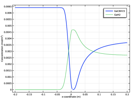
In the Settings window for 1D Plot Group, type Concentration profiles GaC6H15 and GaH2 in the Label text field.
|
|
3
|
|
1
|
|
2
|
|
3
|
Click Replace Expression in the upper-right corner of the y-Axis Data section. From the menu, choose Component 2 (comp2)>Transport of Diluted Species>Species cGaC6H15>cGaC6H15 - Concentration - mol/m³.
|
|
4
|
Click Replace Expression in the upper-right corner of the x-Axis Data section. From the menu, choose Component 2 (comp2)>Geometry>Coordinate>x - x-coordinate.
|
|
5
|
|
6
|
|
7
|
|
1
|
In the Model Builder window, right-click Concentration profiles GaC6H15 and GaH2 and choose Line Graph.
|
|
2
|
|
3
|
Click Replace Expression in the upper-right corner of the y-Axis Data section. From the menu, choose Component 2 (comp2)>Transport of Diluted Species>Species cGaH2>cGaH2 - Concentration - mol/m³.
|
|
4
|
Click Replace Expression in the upper-right corner of the x-Axis Data section. From the menu, choose Component 2 (comp2)>Geometry>Coordinate>x - x-coordinate.
|
|
5
|
|
6
|
|
1
|
|
2
|
|
3
|
|
4
|
|
5
|
|
1
|
|
2
|
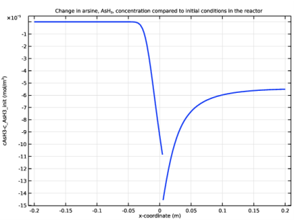
In the Settings window for 1D Plot Group, type Concentration profile AsH3 change in the Label text field.
|
|
3
|
|
1
|
|
2
|
In the Settings window for Line Graph, click Replace Expression in the upper-right corner of the y-Axis Data section. From the menu, choose Component 2 (comp2)>Transport of Diluted Species>Species cAsH3>cAsH3 - Concentration - mol/m³.
|
|
3
|
|
4
|
|
5
|
In the Title text area, type Change in arsine, AsH<sub>3</sub>, concentration compared to initial conditions in the reactor.
|
|
6
|
Click Replace Expression in the upper-right corner of the x-Axis Data section. From the menu, choose Component 2 (comp2)>Geometry>Coordinate>x - x-coordinate.
|
|
7
|
|
8
|
|
1
|
|
2
|
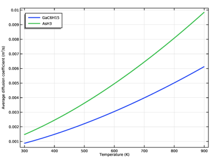
In the Settings window for 1D Plot Group, type Diffusivities vs. temperature in the Label text field.
|
|
3
|
|
1
|
|
2
|
|
3
|
Click Replace Expression in the upper-right corner of the y-Axis Data section. From the menu, choose Component 2 (comp2)>Transport of Diluted Species>Species cGaC6H15>tds.Dav_cGaC6H15 - Average diffusion coefficient - m²/s.
|
|
4
|
|
5
|
Click Replace Expression in the upper-right corner of the x-Axis Data section. From the menu, choose Component 2 (comp2)>Heat Transfer in Fluids>Temperature>T - Temperature - K.
|
|
6
|
|
7
|
|
8
|
|
10
|
|
1
|
|
2
|
|
3
|
Click Replace Expression in the upper-right corner of the y-Axis Data section. From the menu, choose Component 2 (comp2)>Transport of Diluted Species>Species cAsH3>tds.Dav_cAsH3 - Average diffusion coefficient - m²/s.
|
|
4
|
|
5
|
Click Replace Expression in the upper-right corner of the x-Axis Data section. From the menu, choose Component 2 (comp2)>Heat Transfer in Fluids>Temperature>T - Temperature - K.
|
|
6
|
|
7
|
|
8
|
|
1
|
|
2
|
|
3
|
|
4
|
|
5
|
|
6
|
|
7
|
|
8
|
|
1
|
|
2
|
|
3
|
|
1
|
|
2
|
In the Settings window for Line Graph, click Replace Expression in the upper-right corner of the y-Axis Data section. From the menu, choose Component 2 (comp2)>Heat Transfer in Fluids>Material properties>ht.kmean - Mean effective thermal conductivity - W/(m·K).
|
|
3
|
|
4
|
Click Replace Expression in the upper-right corner of the x-Axis Data section. From the menu, choose Component 2 (comp2)>Heat Transfer in Fluids>Temperature>T - Temperature - K.
|
|
5
|
|
1
|
|
2
|
|
3
|
|
4
|