
|
|
|
|
1
|
|
2
|
|
3
|
Click Add.
|
|
4
|
Click
|
|
5
|
|
6
|
Click
|
|
1
|
|
2
|
|
3
|
|
4
|
Browse to the model’s Application Libraries folder and double-click the file dna_degradation_parameters.txt.
|
|
1
|
|
2
|
|
3
|
|
1
|
|
2
|
|
3
|
|
1
|
|
2
|
|
3
|
|
1
|
|
2
|
|
3
|
|
1
|
|
2
|
|
3
|
|
4
|
|
1
|
|
2
|
|
3
|
In the Parameter table, enter the following settings:
|
|
4
|
Click
|
|
5
|
In the Parameter table, enter the following settings:
|
|
6
|
Click
|
|
7
|
In the Parameter table, enter the following settings:
|
|
8
|
Click
|
|
9
|
In the Parameter table, enter the following settings:
|
|
1
|
|
2
|
|
3
|
Click Browse.
|
|
4
|
Browse to the model’s Application Libraries folder and double-click the file dna_degradation_experiment1.csv.
|
|
5
|
Click Import.
|
|
1
|
|
2
|
|
1
|
|
2
|
|
3
|
|
1
|
|
2
|
|
3
|
|
1
|
|
2
|
|
3
|
|
1
|
|
2
|
|
3
|
|
1
|
|
2
|
|
3
|
|
4
|
|
5
|
|
6
|
|
1
|
|
2
|
|
3
|
|
4
|
|
5
|
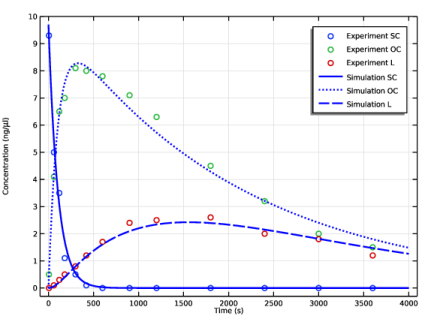
In the associated text field, type Time (s).
|
|
6
|
|
7
|
In the associated text field, type Concentration (ng/\mu l).
|
|
1
|
|
2
|
|
3
|
|
1
|
|
2
|
|
3
|
Click Replace Expression in the upper-right corner of the y-Axis Data section. From the menu, choose Component 1 (comp1)>Reaction Engineering>re.c_SC - Concentration - mol/m³.
|
|
4
|
Click Add Expression in the upper-right corner of the y-Axis Data section. From the menu, choose Component 1 (comp1)>Reaction Engineering>re.c_OC - Concentration - mol/m³.
|
|
5
|
Click Add Expression in the upper-right corner of the y-Axis Data section. From the menu, choose Component 1 (comp1)>Reaction Engineering>re.c_L - Concentration - mol/m³.
|
|
6
|
Click to expand the Coloring and Style section. Find the Line style subsection. From the Line list, choose Cycle.
|
|
7
|
|
8
|
|
9
|
|
11
|
|
12
|
|
13
|