PDF

Chemical Reactions and Soot Build-Up in a Diesel Filter
Introduction
This example deals with a model of a filter system for a diesel engine. A porous filter separates soot particles from exhaust gases passing through it, leading to the formation of a soot layer. Both catalytic and non-catalytic reactions suppress the layer’s build-up; carbon is oxidized to carbon monoxide and carbon dioxide, which both pass through the membrane.
Diesel filters are used to remove particulate matter in diesel-engine exhaust gases. A filter system’s efficiency and durability are closely related to the manner in which it removes soot deposits from the porous filter walls. For instance, one method is to remove the soot layer by means of non-catalytic reactions with oxygen. However, this scheme requires that the exhaust temperature is increased above normal operating conditions. Another approach involves introducing cerium additives to the fuel. Cerium oxide species are subsequently present in the soot layer, acting as a catalyst in carbon-oxidation reactions. Under these conditions, it is possible to remove carbon deposits in the filter without increasing the exhaust temperature. The following model illustrates both of these working conditions.
Diesel filters are typically of a monolithic type with narrow channels running through a cylindrical structure. The silicon carbide filter under study is 15 cm long with a total of 2000 channels. Filter channels are open only at one end and are arranged in an alternating fashion in the monolith. The channels are separated by porous walls, as illustrated in Figure 1.
Figure 1: Front view of a channel section in a diesel filter. The A-channels are open while the B-channels are closed (from the left). The channels are separated by porous filter walls. A back view would show the opposite configuration. Gas enters the filter through the A-channels and exits through the B-channels.
This application follows a two-part strategy to investigate the system in which these reactions take place. The first part is setting up an ideal model in the Reaction Engineering interface with the plug-flow reactor feature that assumes stationary conditions and accounts only for variations with reactor volume. This gives a rather qualitative understanding of the reactor system. The second part sets up a space- and time-dependent model in which variations in species composition, soot layer build up, and temperature are investigated in detail.
Model Definition
Chemical Reactions
The soot layer in the diesel filter must be removed continuously or at intervals to keep the filter in working condition. Oxygen can react with carbon to form carbon monoxide and carbon dioxide. Further reaction pathways open when the diesel fuel is treated with additives containing cerium. The soot layer then contains cerium-oxide species that act as catalysts to oxidize the carbon, and oxygen regenerates the catalyst.
This model considers the following five reactions
(1)
(2)
(3)
(4)
(5)
where (s) indicate a solid phase species.
The reactions are assumed to only occur in the soot layer. The reaction rates (mol/(m3·s)) are given by:
where cO2 is the molar concentration of oxygen (SI unit: mol/m3), while xCeO2 and xCe2O3 are the molar fractions of the different cerium (catalytic) species.
Plug FLOW MODEL
The Reaction Engineering interface can automatically define the material and energy balances for a plug-flow reactor at steady-state, as shown by the governing equation:
(6)
Fi is the molar flow and Ri  includes all the reactions, per unit volume of the channel, in which species i is involved. Equation 6 thus gives a solution of an ideal model system only dependent on the accumulated volume, V, the species pass in the reactor. The plug flow model is solved for isothermal conditions assuming the reactions have negligible impact on temperature in the system since it contains an excess of nitrogen solvent.
The modeled system is schematically illustrated in Figure 2 and consists of one single cell and one single filter-unit. The exhaust gas enters Channel A and passes through a single filter wall to Channel B (note that a repetitive cell would have a filter wall on all sides). The plug flow model system treats just Channel A, the deposited particles, and the catalyst, and neglects any reaction in Channel B. Along the system boundaries, the filter is a distributed outlet. Because the pressure loss over the filter wall is comparably large, the velocity across the wall along the length of the channel is considered to be constant. This implies that the velocity component along the channel decreases linearly from the inlet to the outlet.
Figure 2: Schematic illustration the plug flow system. The exhaust enters Channel A, goes through the filter wall, and exits through Channel B. Assume the velocity across the filter wall is constant along the x direction in the plug flow model, while the velocity component along the length of the channel decreases linearly with the distance from the inlet.
The general material balance for a small section of Channel A of length Δx gives the following equation for any species i:
(7)
Ni denotes the flux vector (mol/(m2s)), Acs equals the channel’s cross-sectional area (m2), L the reactor length (m), and uf represents the velocity flow of species toward the filter (m/s). At ideal conditions, Equation 7 can likewise be set up over the volume element (ΔV) through which the gas passes in Δx:
(8)
In Equation 8, vf represents a volumetric flow of species toward the filter (SI unit: m3/s), H the reactor height (SI unit: m). The reaction is limited to the soot layer on the filter surface. Because the kinetic data is given per unit volume of soot, the volume of soot per unit is estimated to be the same as the volume of the channel. Dividing Equation 8 by ΔV and if ΔV approaches zero gives:
(9)
From the assumption of a linearly decreasing flow along the channel, the volumetric flow in the reactor is given by:
where ku (1/s) denotes the proportionality constant and v0 (m3/s) equals the inlet flow. V is the accumulated volume the species have passed in the tubular reactor. Note that the cross-sectional area is actually irrelevant; that is, the reactor volume, V, can just as well be interpreted as length and compositions, ci, as mol per reactor length. The second term on the left-hand side in Equation 9 is added to all species in the model using the Additional Source feature. The compositions of species along the plug-flow reactor are expressed in terms of concentrations with inlet molar flows set as a simplification for all species. Another generalization is that all species are affected by the flow over the filter, even the solid components.
Space-Dependent Model
This example removes a channel section from the monolith and places it into an experimental setup to study only a single filter unit with a single filter wall. Assuming that only a single filter wall exists and by thermally and mechanically insulating the upper and vertical channel walls, the system can be described with the 2D geometry shown in Figure 3.
Figure 3: Modeled domain including four sections: the inlet Channel A, soot layer, filter wall, and outlet Channel B. Note that the units on the horizontal and vertical axes are different.
The model includes four model sections: the inlet Channel A, the soot layer on the surface of the filter wall, the filter wall, and the outlet Channel B.
The filter is 15 cm long, and the height of a single channel is 1.27 mm. The filter wall is 0.45 mm thick. Diesel exhaust gas enters the inlet channel, and the gas containing soot particles filters off through the porous SiC filter wall, thereby leaving a soot layer on top of this wall. The exhaust exits the filter through the outlet channel. You must treat the top surface of the soot layer as a moving sub-boundary that grows and shrinks according to the amount of soot.
To solve this model, use the following physics interfaces in the space-dependent model:
The position of the top boundary is solved for using the Moving Mesh feature.
In the Free and Porous Media Flow interface, free flow is defined in both the inlet (A) and outlet (B) channels, whereas the Porous Matrix Properties are defined in the soot layer and the filter wall. The reaction kinetics are defined from the plug flow using the Generate Space-Dependent Model feature. This creates a a Chemistry interface to be used in the space-dependent model.
There are two issues worth mentioning regarding the domain equations and boundary conditions used in the model implementation:
Here, vn is normal velocity of the mesh, ρsoot is the density of the soot layer and ρpart is density of the gas phase particles. The first term on the right hand side corresponds to the transport of soot particles towards the soot layer. The second term represents the removal of soot due to reactions inside the layer. Here Mc equals the molar weight of carbon, Rc is the sum of all carbon-consuming reaction rates, and δsl is the soot layer thickness. In the model the reaction rates are assumed to be constant throughout the soot layer. This assumption can also be validated from the results.
where ρmix is the mixture’s density (SI unit: kg/m3), Cp,mix is its heat capacity (J/(kg·K)), kmix equals its thermal conductivity (W/(m·K)), and εsolid the void fraction (porosity).
Results and Discussion
Chemical Reactions and Plug Flow Model
Start by looking at the plug flow model for Channel A. Figure 4 and Figure 5 depict the composition of the reacting species along the channel length at two different temperatures, one at 653 K, below “catalyzer ignition” temperature, and one at 705 K where the catalyst is ignited.
Figure 4: Composition of reacting species along the length of the reactor at 653 K.
Figure 5: Composition along the length of the reactor at 703 K.
At 703 K oxygen becomes depleted at approximately 0.12 m into the reactor. As the temperature increases, the rate of oxidation increases until the depletion of oxygen in the reactor. This decreases the rate of CeO2 regeneration substantially and Ce2O3 becomes the dominating cerium-containing species.
The impact of temperature can also be investigated with the ratio of the non-catalyzed to the catalyzed reaction rates for the carbon monoxide and carbon dioxide producing reactions. In the following figures the reaction rate ratios r1/r3, carbon dioxide production, and r2/r4, carbon monoxide production, rates are depicted for the two different temperatures.
Figure 6: Relationship between the non-catalytic and catalytic carbon-oxidation reactions.
Figure 6 shows that the catalytic reactions by far dominate the oxidation of carbon. This is expected at these relatively moderate temperatures. The oxidation of carbon to carbon dioxide has a higher fraction of non-catalyzed oxidation than that of carbon to carbon monoxide. The dominance of the catalytic reactions decreases with temperature.
Space-Dependent Model
Figure 7 shows the velocity distribution in the channel unit cell at the last time step. The flow is shown to exhibit a laminar behavior.
Figure 7: Velocity magnitude in a filter unit cell.
Figure 8 shows the pressure distribution across the channel pair. The main pressure drop is observed across the soot layer deposited on top of the porous membrane.
Figure 8: Pressure distribution in a filter unit cell.
The oxidation of carbon is overall an exothermic reaction, although the catalytic steps are endothermic. The regeneration of the catalyst is heavily exothermic and makes up for the endothermic properties of the catalytic oxidation reaction. Figure 9 shows the temperature distribution in the system after 1800 s for an inlet temperature of 550 K. The exhaust gases leave the filter at somewhat slightly reduced temperatures due to the net endothermicity of the reactions.
Figure 9: Temperature distribution in the filter for an inlet temperature of 550 K.
The following illustration (Figure 10) shows the soot layer along the length of the reactor at an inlet temperature of 550 K. The base-line corresponds to the initial soot layer thickness of 50 μm. Under the present conditions, carbon oxidation is not sufficient to keep the soot layer from growing. It is also seen that the soot layer build-up is slightly faster at the far end of the filter.
Figure 10: The soot layer’s thickness at 0 to 1800 s in 300 s intervals for an inlet temperature of 550 K.
A fixed outlet pressure is used in the simulation. Figure 10 shows the development of the average inlet pressure. As was seen in Figure 8, the main pressure drop occurs in the compact soot layer. Consequently, the required inlet pressure also increases over time.
Figure 11: Average inlet pressure as a function of time for an inlet temperature of 550 K.
Reference
1. G. Konstantas and A.M. Stamatelos, “Computer Aided Engineering of Diesel Filter Systems,” Joint Meeting of the Greek and Italian Sections of the Combustion Institute, http://www.mie.uth.gr/labs/ltte/pubs/Combust_Inst_Corfou_013.pdf.
Application Library path: Chemical_Reaction_Engineering_Module/Reactors_with_Porous_Catalysts/diesel_filter
Modeling Instructions
From the File menu, choose New.
New
In the New window, click  Model Wizard.
Model Wizard
1
In the Model Wizard window, click  0D.
2
In the Select Physics tree, select Chemical Species Transport>Reaction Engineering (re).
3
Click Add.
4
Click  Study.
5
In the Select Study tree, select Preset Studies for Selected Physics Interfaces>Stationary Plug Flow.
6
Global Definitions
Load model parameters from a text file.
Parameters 1
1
In the Model Builder window, under Global Definitions click Parameters 1.
2
In the Settings window for Parameters, locate the Parameters section.
3
Click  Load from File.
4
Definitions
Variables 1
1
In the Model Builder window, under Component 1 (comp1) right-click Definitions and choose Variables.
Add the variable for the volumetric flow in the tubular reactor.
2
In the Settings window for Variables, locate the Variables section.
3
Reaction Engineering (re)
1
In the Model Builder window, under Component 1 (comp1) click Reaction Engineering (re).
2
In the Settings window for Reaction Engineering, locate the Reactor section.
3
From the Reactor type list, choose Plug flow.
4
Locate the Energy Balance section. In the T text field, type T0.
In order to be able to prescribe the volumetric flow rate, select to compute pressure from the ideal gas law.
5
Locate the Mixture Properties section. From the Reactor pressure list, choose Ideal gas law.
6
Click to expand the Calculate Transport Properties section. Select the Calculate mixture properties check box.
7
Locate the Reactor section. Find the Mass balance subsection. In the v text field, type v1.
Reaction 1
1
In the Reaction Engineering toolbar, click  Reaction.
2
In the Settings window for Reaction, locate the Reaction Formula section.
3
In the Formula text field, type C(s)+O2=>CO2.
4
Click Apply.
Modify the reaction rates in order to take the difference in domain thickness between the catalyzing layer (0.05 mm thick) and the channel (1.27 mm) into account. This is achieved by multiplying all reaction rates with the constant Sa. Alternatively, edit the Arrhenius parameter for the Frequency factor by multiplying the value with the constant Sa.
5
Locate the Rate Constants section. Select the Use Arrhenius expressions check box.
6
In the Af text field, type 1e13[m/s]*Sa.
7
In the Ef text field, type 165e3[J/mol].
8
Locate the Reaction Rate section. From the list, choose User defined.
9
In the rj text field, type re.kf_1*re.c_O2.
10
Find the Volumetric overall reaction order subsection. In the Forward text field, type 1.
In this model, user-defined reaction rate expressions are used.
Reaction 2
1
In the Reaction Engineering toolbar, click  Reaction.
2
In the Settings window for Reaction, locate the Reaction Formula section.
3
In the Formula text field, type C(s)+0.5O2=>CO.
4
Click Apply.
5
Locate the Rate Constants section. Select the Use Arrhenius expressions check box.
6
In the Af text field, type 5.5e10[m/s]*Sa.
7
In the Ef text field, type 150e3[J/mol].
8
Locate the Reaction Rate section. In the rj text field, type re.kf_2*re.c_O2.
9
Find the Volumetric overall reaction order subsection. In the Forward text field, type 1.
Reaction 3
1
In the Reaction Engineering toolbar, click  Reaction.
2
In the Settings window for Reaction, locate the Reaction Formula section.
3
In the Formula text field, type C(s)+4CeO2(s)=>2Ce2O3(s)+CO2.
4
Click Apply.
5
Locate the Rate Constants section. Select the Use Arrhenius expressions check box.
6
In the Af text field, type 4.5e11[m/s]*Sa.
7
In the Ef text field, type 120e3[J/mol].
8
Locate the Reaction Rate section. From the list, choose User defined.
9
In the rj text field, type re.kf_3*re.c_CeO2_solid.
10
Find the Volumetric overall reaction order subsection. In the Forward text field, type 1.
Reaction 4
1
In the Reaction Engineering toolbar, click  Reaction.
2
In the Settings window for Reaction, locate the Reaction Formula section.
3
In the Formula text field, type C(s)+2CeO2(s)=>Ce2O3(s)+CO.
4
Click Apply.
5
Locate the Rate Constants section. Select the Use Arrhenius expressions check box.
6
In the Af text field, type 4e8[m/s]*Sa.
7
In the Ef text field, type 80e3[J/mol].
8
Locate the Reaction Rate section. From the list, choose User defined.
9
In the rj text field, type re.kf_4*re.c_CeO2_solid.
10
Find the Volumetric overall reaction order subsection. In the Forward text field, type 1.
Reaction 5
1
In the Reaction Engineering toolbar, click  Reaction.
2
In the Settings window for Reaction, locate the Reaction Formula section.
3
In the Formula text field, type Ce2O3(s)+0.5O2=>2CeO2(s).
4
Click Apply.
5
Locate the Rate Constants section. Select the Use Arrhenius expressions check box.
6
In the Af text field, type 1e12[m^4/(mol*s)]*Sa.
7
In the Ef text field, type 80e3[J/mol].
8
Locate the Reaction Rate section. In the rj text field, type re.kf_5*re.c_O2*re.c_Ce2O3_solid.
9
Find the Volumetric overall reaction order subsection. In the Forward text field, type 2.
Species: C(s)
The carbon composition is locked in the model.
1
In the Model Builder window, click Species: C(s).
2
In the Settings window for Species, click to expand the Species Concentration/Activity section.
3
Select the Constant concentration/activity check box.
Note that the molar mass of carbon has been set, since we have named the Species using its chemical formula.
Nitrogen is also present in the gas as an inert.
Species 1
1
In the Reaction Engineering toolbar, click  Species.
Constant pressure in channel A is assumed. N2 is simply inert and does not act as a solvent in the first part of the model.
2
In the Settings window for Species, locate the Species Name section.
3
Initial Values 1
1
In the Model Builder window, click Initial Values 1.
2
In the Settings window for Initial Values, locate the Volumetric Species Initial Values section.
3
Additional Source 1
1
In the Reaction Engineering toolbar, click  Additional Source.
All species are driven toward or through the filter as a simplification.
2
In the Settings window for Additional Source, locate the Additional Rate Expression section.
3
In the Volumetric species table, enter the following settings:
Study 1
Step 1: Stationary Plug Flow
1
In the Model Builder window, under Study 1 click Step 1: Stationary Plug Flow.
2
In the Settings window for Stationary Plug Flow, locate the Study Settings section.
3
In the Output volumes text field, type 0.149.
Using 0.149 avoids describing the stagnant zone close to the dead-end of the tubular reactor.
To study the model at two different temperatures, use a parametric sweep to vary T0.
Parametric Sweep
1
In the Study toolbar, click  Parametric Sweep.
2
In the Settings window for Parametric Sweep, locate the Study Settings section.
3
4
5
In the Study toolbar, click  Compute.
Results
Concentrations plug flow model
To produce the plots shown in Figure 4, Figure 5, and Figure 6 follow these steps.
1
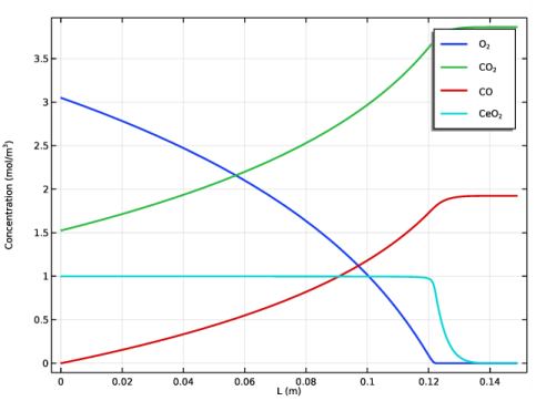
In the Settings window for 1D Plot Group, type Concentrations plug flow model in the Label text field.
2
Click to expand the Title section. From the Title type list, choose None.
3
Locate the Plot Settings section. In the x-axis label text field, type L (m).
Global 1
1
In the Model Builder window, expand the Concentrations plug flow model node, then click Global 1.
2
In the Settings window for Global, locate the Data section.
3
From the Dataset list, choose Study 1/Parametric Solutions 1 (sol2).
4
Locate the y-Axis Data section. In the table, enter the following settings:
5
6
Click  Delete.
7
Click  Delete.
8
Click to expand the Coloring and Style section. In the Width text field, type 2.
9
Click to expand the Legends section. From the Legends list, choose Manual.
10
11
Locate the Data section. From the Parameter selection (T0) list, choose First.
12
In the Concentrations plug flow model toolbar, click  Plot.
13
From the Parameter selection (T0) list, choose Last.
14
In the Concentrations plug flow model toolbar, click  Plot.
Rate comparison plug flow model
1
In the Model Builder window, right-click Concentrations plug flow model and choose Duplicate.
2
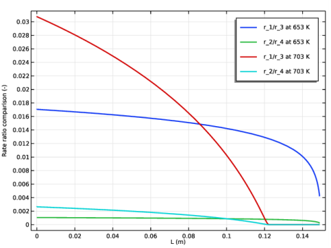
In the Settings window for 1D Plot Group, type Rate comparison plug flow model in the Label text field.
3
Locate the Plot Settings section. Select the y-axis label check box.
4
In the associated text field, type Rate ratio comparison (-).
Global 1
1
In the Model Builder window, expand the Rate comparison plug flow model node, then click Global 1.
2
In the Settings window for Global, locate the Data section.
3
From the Parameter selection (T0) list, choose First.
4
Click Replace Expression in the upper-right corner of the y-Axis Data section. From the menu, choose Component 1 (comp1)>Reaction Engineering>re.r_1 - Reaction rate - mol/(m³·s).
5
Locate the y-Axis Data section. In the table, enter the following settings:
6
Locate the Legends section. In the table, enter the following settings:
Global 2
1
Right-click Results>Rate comparison plug flow model>Global 1 and choose Duplicate.
Use the Generate Space-Dependent Model feature to generate a 2D model that solves mass, energy, and momentum balances within the system.
2
In the Settings window for Global, locate the Data section.
3
From the Parameter selection (T0) list, choose Last.
4
Locate the Legends section. In the table, enter the following settings:
5
In the Rate comparison plug flow model toolbar, click  Plot.
Reaction Engineering (re)
Generate Space-Dependent Model 1
1
In the Reaction Engineering toolbar, click  Generate Space-Dependent Model.
2
In the Settings window for Generate Space-Dependent Model, locate the Component Settings section.
3
From the Component to use list, choose 2D: New.
4
Locate the Physics Interfaces section. Find the Heat transfer subsection. From the list, choose Heat Transfer in Fluids: New.
5
Find the Fluid flow subsection. From the list, choose Free and Porous Media Flow: New.
6
Locate the Space-Dependent Model Generation section. Click Create/Refresh.
Component 2 (comp2)
Also add multiphysics coupling features. These ensure that the coupled interfaces are set up in consistent manner.
Multiphysics
In the Model Builder window, expand the Component 2 (comp2) node, then click Multiphysics.
Nonisothermal Flow 1 (nitf1)
In the Physics toolbar, click  Multiphysics Couplings and choose Domain>Nonisothermal Flow.
Reacting Flow, Diluted Species 1 (rfd1)
In the Physics toolbar, click  Multiphysics Couplings and choose Domain>Reacting Flow, Diluted Species.
The geometry to be used has a high aspect ratio. The length of the geometry is about 50 time the height. In this case using an automatic scaling of the view makes it easier to setup the model. This is since the entire geometry is fitted in the Graphics window.
Definitions (comp2)
In the Model Builder window, expand the Component 2 (comp2)>Definitions node.
Axis
1
In the Model Builder window, expand the Component 2 (comp2)>Definitions>View 1 node, then click Axis.
2
In the Settings window for Axis, locate the Axis section.
3
From the View scale list, choose Automatic.
Geometry 1(2D)
Start by drawing the Outlet Channel, B, as shown in Figure 3.
Rectangle 1 (r1)
1
In the Geometry toolbar, click  Rectangle.
2
In the Settings window for Rectangle, locate the Size and Shape section.
3
In the Width text field, type L+1[cm].
4
In the Height text field, type H.
Next, draw the soot layer and filter wall as follows.
Rectangle 2 (r2)
1
In the Geometry toolbar, click  Rectangle.
2
In the Settings window for Rectangle, locate the Size and Shape section.
3
In the Width text field, type L.
4
In the Height text field, type Hf+dHs.
5
Locate the Position section. In the y text field, type H.
6
Click to expand the Layers section. In the table, enter the following settings:
7
Click  Build Selected.
Rectangle 3 (r3)
1
In the Geometry toolbar, click  Rectangle.
2
In the Settings window for Rectangle, locate the Size and Shape section.
3
In the Width text field, type L.
4
In the Height text field, type 0.5*dHs.
5
Locate the Position section. In the y text field, type H+Hf+dHs.
6
Click  Build Selected.
Finally move the Rectangle 1 as shown below to create the inlet channel.
Move 1 (mov1)
1
In the Geometry toolbar, click  Transforms and choose Move.
2
Click the  Zoom Extents button in the Graphics toolbar.
3
4
In the Settings window for Move, locate the Input section.
5
Select the Keep input objects check box.
6
Locate the Displacement section. In the x text field, type -1[cm].
7
In the y text field, type H+Hf+1.5*dHs.
Form Union (fin)
1
In the Model Builder window, click Form Union (fin).
2
In the Settings window for Form Union/Assembly, click  Build Selected.
3
Click the  Zoom Extents button in the Graphics toolbar.
Make geometry selections.
Inlet
1
In the Geometry toolbar, click  Selections and choose Explicit Selection.
2
In the Settings window for Explicit Selection, type Inlet in the Label text field.
3
Locate the Entities to Select section. From the Geometric entity level list, choose Boundary.
4
On the object fin, select Boundary 1 only.
Outlet
1
In the Geometry toolbar, click  Selections and choose Explicit Selection.
2
In the Settings window for Explicit Selection, type Outlet in the Label text field.
3
Locate the Entities to Select section. From the Geometric entity level list, choose Boundary.
4
On the object fin, select Boundary 18 only.
Channel A
1
In the Geometry toolbar, click  Selections and choose Explicit Selection.
2
In the Settings window for Explicit Selection, type Channel A in the Label text field.
3
On the object fin, select Domains 1 and 5 only.
Soot layer
1
In the Geometry toolbar, click  Selections and choose Explicit Selection.
2
In the Settings window for Explicit Selection, type Soot layer in the Label text field.
3
On the object fin, select Domain 4 only.
Filter wall
1
In the Geometry toolbar, click  Selections and choose Explicit Selection.
2
In the Settings window for Explicit Selection, type Filter wall in the Label text field.
3
On the object fin, select Domain 3 only.
Soot and filter wall
1
In the Geometry toolbar, click  Selections and choose Union Selection.
2
In the Settings window for Union Selection, locate the Input Entities section.
3
4
In the Add dialog box, in the Selections to add list, choose Soot layer and Filter wall.
5
6
In the Settings window for Union Selection, type Soot and filter wall in the Label text field.
Channel B
1
In the Geometry toolbar, click  Selections and choose Explicit Selection.
2
In the Settings window for Explicit Selection, type Channel B in the Label text field.
3
On the object fin, select Domain 2 only.
Global Definitions
Material 1 (mat1)
In the Model Builder window, under Global Definitions right-click Materials and choose Blank Material.
Material 2 (mat2)
Right-click Materials and choose Blank Material.
Materials
Porous Material 1 (poromat1)
1
In the Model Builder window, under Component 2 (comp2) right-click Materials and choose More Materials>Porous Material.
2
Fluid 1 (poromat1.fluid1)
1
Right-click Porous Material 1 (poromat1) and choose Fluid.
2
In the Settings window for Fluid, locate the Fluid Properties section.
3
From the Material list, choose None.
Solid 1 (poromat1.solid1)
1
In the Model Builder window, right-click Porous Material 1 (poromat1) and choose Solid.
2
In the Settings window for Solid, locate the Solid Properties section.
3
In the θs text field, type 1-poro.
Porous Material 2 (poromat2)
1
Right-click Porous Material 1 (poromat1) and choose Duplicate.
2
Solid 1 (poromat2.solid1)
1
In the Model Builder window, expand the Porous Material 2 (poromat2) node, then click Solid 1 (poromat2.solid1).
2
In the Settings window for Solid, locate the Solid Properties section.
3
From the Material list, choose Material 2 (mat2).
Most reaction kinetics definitions were set up in the Reaction Engineering interface, but some changes need to be done directly in the Chemistry interface.
Chemistry 1 (chem)
Adjust the reaction kinetics.
1: C(s)+O2=>CO2
1
In the Model Builder window, expand the Component 2 (comp2)>Chemistry 1 (chem) node, then click 1: C(s)+O2=>CO2.
2
In the Settings window for Reaction, locate the Rate Constants section.
3
In the Af text field, type 1e13.
4
Locate the Reaction Thermodynamic Properties section. From the Enthalpy of reaction list, choose User defined.
5
In the H text field, type -3.96e5[J/mol].
Set the parameters necessary to compute mixture transport properties. Also, the additional source should be inactivated here, since the filter is now included in the model geometry.
Species: O2
1
In the Model Builder window, click Species: O2.
2
In the Settings window for Species, click to expand the Additional Source section.
3
Clear the Additional source check box.
4
Click to expand the Species Transport Expressions section. In the σ text field, type 3.467[angstrom].
5
In the ε/kb text field, type 106.7[K].
Species: CO2
1
In the Model Builder window, click Species: CO2.
2
In the Settings window for Species, locate the Additional Source section.
3
Clear the Additional source check box.
4
Locate the Species Transport Expressions section. In the σ text field, type 3.941[angstrom].
5
In the ε/kb text field, type 195.2[K].
2: C(s)+0.5O2=>CO
1
In the Model Builder window, click 2: C(s)+0.5O2=>CO.
2
In the Settings window for Reaction, locate the Rate Constants section.
3
In the Af text field, type 5.5e10.
4
Locate the Reaction Thermodynamic Properties section. From the Enthalpy of reaction list, choose User defined.
5
In the H text field, type -1.1e5[J/mol].
Species: CO
1
In the Model Builder window, click Species: CO.
2
In the Settings window for Species, locate the Additional Source section.
3
Clear the Additional source check box.
4
Locate the Species Transport Expressions section. In the σ text field, type 3.69[angstrom].
5
In the ε/kb text field, type 91.7[K].
3: C(s)+4CeO2(s)=>2Ce2O3(s)+CO2
1
In the Model Builder window, click 3: C(s)+4CeO2(s)=>2Ce2O3(s)+CO2.
2
In the Settings window for Reaction, locate the Rate Constants section.
3
In the Af text field, type 4.5e11.
4
Locate the Reaction Thermodynamic Properties section. From the Enthalpy of reaction list, choose User defined.
5
In the H text field, type 6.72e4[J/mol].
The concentration of the cerium additatives are assumed to be constant in the space-dependent model.
Species: CeO2(s)
1
In the Model Builder window, click Species: CeO2(s).
2
In the Settings window for Species, click to expand the Species Concentration/Activity section.
3
Select the Constant concentration/activity check box.
Species: Ce2O3(s)
1
In the Model Builder window, click Species: Ce2O3(s).
2
In the Settings window for Species, locate the Species Concentration/Activity section.
3
Select the Constant concentration/activity check box.
4: C(s)+2CeO2(s)=>Ce2O3(s)+CO
1
In the Model Builder window, click 4: C(s)+2CeO2(s)=>Ce2O3(s)+CO.
2
In the Settings window for Reaction, locate the Rate Constants section.
3
In the Af text field, type 4e8.
4
Locate the Reaction Thermodynamic Properties section. From the Enthalpy of reaction list, choose User defined.
5
In the H text field, type 1.21e5[J/mol].
5: Ce2O3(s)+0.5O2=>2CeO2(s)
1
In the Model Builder window, click 5: Ce2O3(s)+0.5O2=>2CeO2(s).
2
In the Settings window for Reaction, locate the Rate Constants section.
3
In the Af text field, type 1e12.
4
Locate the Reaction Thermodynamic Properties section. From the Enthalpy of reaction list, choose User defined.
5
In the H text field, type -2.24e5[J/mol].
Select nitrogen as a solvent. When a species has been selected as solvent, the physical properties of the mixture will be defined from the solvent. This fits the Transport in Diluted Species interface particularly well.
Additionally, add the thermodynamic properties for the solvent.
Species: N2
1
In the Model Builder window, click Species: N2.
2
In the Settings window for Species, locate the Species Type section.
3
4
Locate the Species Transport Expressions section. In the σ text field, type 3.798[angstrom].
5
In the ε/kb text field, type 71.4[K].
6
Click to expand the Species Thermodynamic Expressions section. In the Tmid text field, type 3000[K].
7
In the Thi text field, type 3000[K].
8
In the alow,1 text field, type 3.298677.
9
In the alow,2 text field, type 0.14082404e-2.
10
In the alow,3 text field, type -0.03963222e-4.
11
In the alow,4 text field, type 0.05641515e-7.
12
In the alow,5 text field, type -0.02444854e-10.
13
In the alow,6 text field, type -0.10208999e4.
14
In the alow,7 text field, type 3.950372.
Last, set the concentrations of the species not solved for.
15
In the Model Builder window, click Chemistry 1 (chem).
16
In the Settings window for Chemistry, locate the Species Matching section.
17
Find the Bulk species subsection. In the table, enter the following settings:
18
Find the Solid species subsection. In the table, enter the following settings:
Move on to the rest of the interfaces.
Transport of Diluted Species (tds)
1
In the Model Builder window, under Component 2 (comp2) click Transport of Diluted Species (tds).
2
In the Settings window for Transport of Diluted Species, locate the Transport Mechanisms section.
3
Select the Mass transfer in porous media check box.
Remove the species that are not involved in the mass transport: the solid phase species and the solvent.
4
Click to expand the Dependent Variables section. In the Number of species text field, type 3.
5
In the Concentrations table, enter the following settings:
Transport Properties 1
1
In the Model Builder window, expand the Transport of Diluted Species (tds) node, then click Transport Properties 1.
2
In the Settings window for Transport Properties, locate the Diffusion section.
3
From the Source list, choose Chemistry.
4
From the DcO2 list, choose Diffusion coefficient , O2 in N2 (solvent) (chem).
5
From the DcCO2 list, choose Diffusion coefficient , CO2 in N2 (solvent) (chem).
6
From the DcCO list, choose Diffusion coefficient , CO in N2 (solvent) (chem).
Initial Values 1
1
In the Model Builder window, click Initial Values 1.
2
In the Settings window for Initial Values, locate the Initial Values section.
3
In the cO2 text field, type 0.
4
In the cCO2 text field, type 0.
5
In the cCO text field, type 0.
The reactions should only take place in the soot layer.
Reactions 1
1
In the Model Builder window, click Reactions 1.
2
In the Settings window for Reactions, locate the Domain Selection section.
3
From the Selection list, choose Soot layer.
4
Locate the Reaction Rates section. From the RcO2 list, choose Reaction rate for species O2 (chem).
5
From the RcCO list, choose Reaction rate for species CO (chem).
6
Click to expand the Reacting Volume section. From the list, choose Pore volume.
Inflow 1
Set the concentrations at the inflow boundary to be same as the initial concentrations.
1
In the Model Builder window, click Inflow 1.
2
In the Settings window for Inflow, locate the Boundary Selection section.
3
From the Selection list, choose Inlet.
4
Locate the Concentration section. In the c0,cO2 text field, type F_O2_inlet/v_inlet.
5
In the c0,cCO2 text field, type F_CO2_inlet/v_inlet.
6
In the c0,cCO text field, type F_CO_inlet/v_inlet.
Outflow 1
1
In the Model Builder window, click Outflow 1.
2
In the Settings window for Outflow, locate the Boundary Selection section.
3
From the Selection list, choose Outlet.
Porous Medium 1
1
In the Physics toolbar, click  Domains and choose Porous Medium.
2
Fluid 1
1
In the Model Builder window, expand the Porous Medium 1 node, then click Fluid 1.
2
In the Settings window for Fluid, locate the Diffusion section.
3
From the Source list, choose Chemistry.
4
From the DcO2 list, choose Diffusion coefficient , O2 in N2 (solvent) (chem).
5
From the DcCO2 list, choose Diffusion coefficient , CO2 in N2 (solvent) (chem).
6
From the DcCO list, choose Diffusion coefficient , CO in N2 (solvent) (chem).
7
From the Effective diffusivity model list, choose No correction.
Continue with the Heat Transfer in Fluids interface. Note that several properties are available from the Chemistry interface.
Heat Transfer in Fluids 1 (ht)
Initial Values 1
1
In the Model Builder window, under Component 2 (comp2)>Heat Transfer in Fluids 1 (ht) click Initial Values 1.
2
In the Settings window for Initial Values, locate the Initial Values section.
3
In the T text field, type Tin.
Heat Source 1
1
In the Model Builder window, click Heat Source 1.
2
In the Settings window for Heat Source, locate the Domain Selection section.
3
From the Selection list, choose Soot layer.
Temperature 1
1
In the Model Builder window, click Temperature 1.
2
In the Settings window for Temperature, locate the Boundary Selection section.
3
From the Selection list, choose Inlet.
4
Locate the Temperature section. In the T0 text field, type Tin.
Outflow 1
1
In the Model Builder window, click Outflow 1.
2
In the Settings window for Outflow, locate the Boundary Selection section.
3
From the Selection list, choose Outlet.
Porous Medium 1
1
In the Physics toolbar, click  Domains and choose Porous Medium.
2
Fluid 1
1
In the Model Builder window, expand the Porous Medium 1 node, then click Fluid 1.
2
In the Settings window for Fluid, locate the Heat Conduction, Fluid section.
3
From the kf list, choose Thermal conductivity (chem).
4
Locate the Thermodynamics, Fluid section. From the ρf list, choose Density (chem).
5
From the Cp,f list, choose Heat capacity at constant pressure (chem).
6
From the γ list, choose User defined.
Global Definitions
Material 1 (mat1)
1
In the Model Builder window, under Global Definitions>Materials click Material 1 (mat1).
2
In the Settings window for Material, locate the Material Contents section.
3
Material 2 (mat2)
1
In the Model Builder window, click Material 2 (mat2).
2
In the Settings window for Material, locate the Material Contents section.
3
Free and Porous Media Flow 1 (fp)
Inlet 1
1
In the Model Builder window, under Component 2 (comp2)>Free and Porous Media Flow 1 (fp) click Inlet 1.
2
In the Settings window for Inlet, locate the Boundary Selection section.
3
From the Selection list, choose Inlet.
4
Locate the Boundary Condition section. From the list, choose Fully developed flow.
5
Locate the Fully Developed Flow section. In the Uav text field, type 2.5[m/s].
Outlet 1
1
In the Model Builder window, click Outlet 1.
2
In the Settings window for Outlet, locate the Boundary Selection section.
3
From the Selection list, choose Outlet.
4
Locate the Pressure Conditions section. Select the Normal flow check box.
Fluid and Matrix Properties 1
1
In the Physics toolbar, click  Domains and choose Fluid and Matrix Properties.
2
In the Settings window for Fluid and Matrix Properties, locate the Domain Selection section.
3
From the Selection list, choose Soot layer.
4
Locate the Fluid Properties section. From the μ list, choose Dynamic viscosity (chem).
5
Locate the Porous Matrix Properties section. From the εp list, choose User defined. In the associated text field, type poro.
6
From the κ list, choose User defined. In the associated text field, type kappa_s.
Fluid and Matrix Properties 2
1
Right-click Fluid and Matrix Properties 1 and choose Duplicate.
2
In the Settings window for Fluid and Matrix Properties, locate the Domain Selection section.
3
From the Selection list, choose Filter wall.
4
Locate the Porous Matrix Properties section. In the κ text field, type kappa_m.
The soot layer changes in size and the model takes this into account using a Moving Mesh feature. The top of the soot layer (boundary 11) is prescribed to move in accordance with the soot build-up, and the adjacent domains are allowed to change shape.
Definitions (comp2)
Deforming Domain 1
1
In the Definitions toolbar, click  Moving Mesh and choose Deforming Domain.
2
Prescribed Normal Mesh Velocity 1
1
In the Definitions toolbar, click  Moving Mesh and choose Prescribed Normal Mesh Velocity.
2
The soot layer build-up is controlled by the transport of carbon particles to the layer, as well as the consumption of soot particles inside the layer.
3
In the Settings window for Prescribed Normal Mesh Velocity, locate the Prescribed Normal Mesh Velocity section.
4
In the vn text field, type (-paco*(u*fp.nx+v*fp.ny)-Mc*((y-Y)+dHsoot)*(comp2.chem.r_1+comp2.chem.r_2+comp2.chem.r_3+ comp2.chem.r_4))/rho_s.
Prescribed Normal Mesh Displacement 1
1
In the Definitions toolbar, click  Moving Mesh and choose Prescribed Normal Mesh Displacement.
2
3
Click the  Zoom Extents button in the Graphics toolbar.
Next step is to build a suitable mesh. Due to the regular structure of the geometry, a mapped mesh both captures the physics and keeps the number of elements to a minimum.
Mesh 1
Mapped 1
1
In the Mesh toolbar, click  Mapped.
2
In the Settings window for Mapped, locate the Domain Selection section.
3
From the Geometric entity level list, choose Domain.
4
5
Click the  Zoom Extents button in the Graphics toolbar.
Distribution 1
1
Right-click Mapped 1 and choose Distribution.
2
3
In the Settings window for Distribution, locate the Distribution section.
4
From the Distribution type list, choose Predefined.
5
In the Number of elements text field, type 25.
6
In the Element ratio text field, type 3.
7
Select the Symmetric distribution check box.
Distribution 2
1
In the Model Builder window, right-click Mapped 1 and choose Distribution.
2
3
In the Settings window for Distribution, locate the Distribution section.
4
From the Distribution type list, choose Predefined.
5
In the Number of elements text field, type 10.
6
In the Element ratio text field, type 3.
Distribution 3
1
Right-click Mapped 1 and choose Distribution.
2
3
In the Settings window for Distribution, locate the Distribution section.
4
From the Distribution type list, choose Predefined.
5
In the Number of elements text field, type 90.
6
In the Element ratio text field, type 10.
7
Select the Symmetric distribution check box.
Distribution 4
1
Right-click Mapped 1 and choose Distribution.
2
Click the  Zoom Extents button in the Graphics toolbar.
3
In the Settings window for Distribution, locate the Boundary Selection section.
4
Click  Paste Selection.
5
In the Paste Selection dialog box, type 8, 10, 15, 16 in the Selection text field.
6
Distribution 5
1
Right-click Mapped 1 and choose Distribution.
2
3
In the Settings window for Distribution, locate the Distribution section.
4
In the Number of elements text field, type 15.
5
Click  Build Selected.
Mapped 2
In the Mesh toolbar, click  Mapped.
Distribution 1
1
Right-click Mapped 2 and choose Distribution.
2
3
In the Settings window for Distribution, locate the Distribution section.
4
From the Distribution type list, choose Predefined.
5
In the Number of elements text field, type 25.
6
In the Element ratio text field, type 3.
Distribution 2
1
In the Model Builder window, right-click Mapped 2 and choose Distribution.
2
3
In the Settings window for Distribution, locate the Distribution section.
4
From the Distribution type list, choose Predefined.
5
In the Number of elements text field, type 10.
6
In the Element ratio text field, type 3.
7
Click  Build All.
8
Click the  Zoom Extents button in the Graphics toolbar.
Hide the internal boundary just above the soot layer. This was kept in the model to simplify the mesh generation.
Definitions (comp2)
Hide for Physics 1
1
In the Model Builder window, right-click View 1 and choose Hide for Physics.
2
In the Settings window for Hide for Physics, locate the Geometric Entity Selection section.
3
From the Geometric entity level list, choose Boundary.
4
In a model described by a strongly coupled system of equations, it is often a good practice to solve the problem sequentially to avoid convergence issues. Start by solving for the stationary flow. After that, solve the full time-dependent system, with the dynamic nature of the soot layer handled by the Moving Mesh feature.
Study 2
Step 1: Stationary
1
In the Model Builder window, expand the Study 2 node, then click Step 1: Stationary.
2
In the Settings window for Stationary, locate the Physics and Variables Selection section.
3
Time Dependent
1
In the Study toolbar, click  Study Steps and choose Time Dependent>Time Dependent.
2
In the Settings window for Time Dependent, locate the Physics and Variables Selection section.
3
In the table, clear the Solve for check box for Reaction Engineering (re).
4
Locate the Study Settings section. In the Output times text field, type range(0,300,1800).
Set up proportional Scale values for Dependent Variables 2.
Solution 5 (sol5)
1
In the Study toolbar, click  Show Default Solver.
2
In the Model Builder window, expand the Solution 5 (sol5) node.
3
In the Model Builder window, expand the Study 2>Solver Configurations>Solution 5 (sol5)>Dependent Variables 2 node, then click Concentration (comp2.cCO).
4
In the Settings window for Field, locate the Scaling section.
5
From the Method list, choose Manual.
6
In the Model Builder window, click Concentration (comp2.cCO2).
7
In the Settings window for Field, locate the Scaling section.
8
From the Method list, choose Manual.
9
In the Model Builder window, click Concentration (comp2.cO2).
10
In the Settings window for Field, locate the Scaling section.
11
From the Method list, choose Manual.
12
In the Model Builder window, click Temperature (comp2.T).
13
In the Settings window for Field, locate the Scaling section.
14
From the Method list, choose Initial value based.
To avoid discontinuities at the inlet for the Time Dependent study, add a step function to gradually increase the Inflow concentration
Definitions (comp2)
Step 1 (step1)
1
In the Home toolbar, click  Functions and choose Global>Step.
2
In the Settings window for Step, locate the Parameters section.
3
In the Location text field, type 0.5.
4
Click to expand the Smoothing section. In the Size of transition zone text field, type 1.
Transport of Diluted Species (tds)
Inflow 1
1
In the Model Builder window, under Component 2 (comp2)>Transport of Diluted Species (tds) click Inflow 1.
2
In the Settings window for Inflow, locate the Concentration section.
3
In the c0,cO2 text field, type F_O2_inlet/v_inlet*step1(t[1/s]).
4
In the c0,cCO2 text field, type F_CO2_inlet/v_inlet*step1(t[1/s]).
5
In the c0,cCO text field, type F_CO_inlet/v_inlet*step1(t[1/s]).
Study 2
In the Home toolbar, click  Compute.
Results
Streamline 1
1
In the Model Builder window, expand the Results>Concentration, O2 (tds) node, then click Streamline 1.
2
In the Settings window for Streamline, locate the Streamline Positioning section.
3
From the Positioning list, choose On selected boundaries.
4
In the Number text field, type 15.
5
Locate the Selection section. Select the  Activate Selection toggle button.
6
7
Locate the Coloring and Style section. Find the Point style subsection. From the Arrow length list, choose Normalized.
8
Select the Scale factor check box.
9
10
In the Concentration, O2 (tds) toolbar, click  Plot.
Streamline 1
1
In the Model Builder window, expand the Results>Concentration, CO2 (tds) node, then click Streamline 1.
2
In the Settings window for Streamline, locate the Streamline Positioning section.
3
From the Positioning list, choose On selected boundaries.
4
In the Number text field, type 15.
5
Locate the Selection section. Select the  Activate Selection toggle button.
6
7
Locate the Coloring and Style section. Find the Point style subsection. From the Arrow length list, choose Normalized.
8
Select the Scale factor check box.
9
10
In the Concentration, CO2 (tds) toolbar, click  Plot.
Streamline 1
1
In the Model Builder window, expand the Results>Concentration, CO (tds) node, then click Streamline 1.
2
In the Settings window for Streamline, locate the Streamline Positioning section.
3
From the Positioning list, choose On selected boundaries.
4
In the Number text field, type 15.
5
Locate the Selection section. Select the  Activate Selection toggle button.
6
7
Locate the Coloring and Style section. Find the Point style subsection. From the Arrow length list, choose Normalized.
8
Select the Scale factor check box.
9
10
In the Concentration, CO (tds) toolbar, click  Plot.
To produce the plots shown in Figures 7-11 follow these steps.
Surface
1
In the Model Builder window, expand the Results>Velocity (fp1) node, then click Surface.
2
In the Settings window for Surface, locate the Coloring and Style section.
3
From the Color table list, choose Twilight.
4
Select the Reverse color table check box.
5
In the Velocity (fp1) toolbar, click  Plot.
Streamline 1
1
In the Model Builder window, right-click Velocity (fp1) and choose Streamline.
2
In the Settings window for Streamline, click Replace Expression in the upper-right corner of the Expression section. From the menu, choose Component 2 (comp2)>Free and Porous Media Flow 1>Velocity and pressure>u,v - Velocity field (spatial frame).
3
4
Locate the Coloring and Style section. Find the Point style subsection. From the Color list, choose Gray.
5
From the Type list, choose Arrow.
6
Select the Scale factor check box.
7
8
In the Velocity (fp1) toolbar, click  Plot.
9
Click the  Zoom Extents button in the Graphics toolbar.
Contour
1
In the Model Builder window, expand the Pressure (fp1) node.
2
Right-click Contour and choose Disable.
Surface 1
1
In the Model Builder window, right-click Pressure (fp1) and choose Surface.
2
In the Settings window for Surface, locate the Expression section.
3
In the Expression text field, type p.
4
In the Pressure (fp1) toolbar, click  Plot.
Temperature (ht1)
1
In the Model Builder window, click Temperature (ht1).
2
In the Temperature (ht1) toolbar, click  Plot.
3
Click the  Zoom Extents button in the Graphics toolbar.
Soot layer thickness
1
In the Home toolbar, click  Add Plot Group and choose 1D Plot Group.
2
In the Settings window for 1D Plot Group, type Soot layer thickness in the Label text field.
3
Locate the Data section. From the Dataset list, choose Study 2/Solution 5 (sol5).
4
Locate the Title section. From the Title type list, choose None.
5
Locate the Plot Settings section. Select the x-axis label check box.
6
7
Select the y-axis label check box.
8
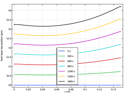
In the associated text field, type Soot layer top position (\mu m).
9
Locate the Legend section. From the Position list, choose Lower middle.
Line Graph 1
1
Right-click Soot layer thickness and choose Line Graph.
2
Click the  Zoom Extents button in the Graphics toolbar.
3
4
In the Settings window for Line Graph, locate the y-Axis Data section.
5
In the Expression text field, type y-Y+dHsoot.
6
From the Unit list, choose µm.
7
Click to expand the Coloring and Style section. In the Width text field, type 2.
8
Click to expand the Legends section. Select the Show legends check box.
9
In the Soot layer thickness toolbar, click  Plot.
10
Click the  Zoom Extents button in the Graphics toolbar.
1D Plot Group 11
1
In the Home toolbar, click  Add Plot Group and choose 1D Plot Group.
2
In the Settings window for 1D Plot Group, locate the Data section.
3
From the Dataset list, choose Study 2/Solution 5 (sol5).
Global 1
1
Right-click 1D Plot Group 11 and choose Global.
2
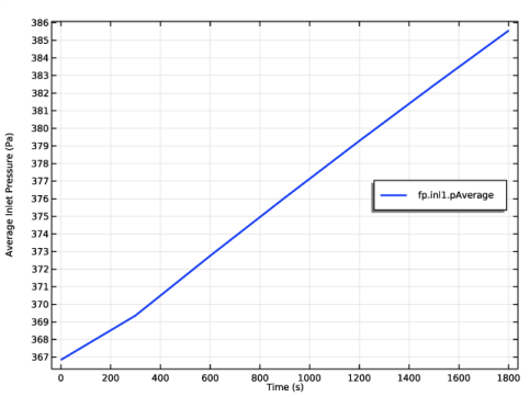
In the Settings window for Global, click Replace Expression in the upper-right corner of the y-Axis Data section. From the menu, choose Component 2 (comp2)>Free and Porous Media Flow 1>Auxiliary variables>fp.inl1.pAverage - Pressure average over feature selection - Pa.
3
Locate the y-Axis Data section. In the table, enter the following settings:
4
Locate the Coloring and Style section. In the Width text field, type 2.
5
In the 1D Plot Group 11 toolbar, click  Plot.
Inlet pressure
1
In the Model Builder window, under Results click 1D Plot Group 11.
2
In the Settings window for 1D Plot Group, type Inlet pressure in the Label text field.
3
Locate the Title section. From the Title type list, choose None.
4
Locate the Legend section. From the Position list, choose Middle right.
5
Click the  Zoom Extents button in the Graphics toolbar.
For future use of Study 1 disable the interfaces that are used in the space-dependent model.
Study 1
Step 1: Stationary Plug Flow
1
In the Model Builder window, under Study 1 click Step 1: Stationary Plug Flow.
2
In the Settings window for Stationary Plug Flow, locate the Physics and Variables Selection section.
3
In the table, clear the Solve for check boxes for Chemistry 1 (chem), Transport of Diluted Species (tds), Heat Transfer in Fluids 1 (ht), Free and Porous Media Flow 1 (fp), and Moving mesh (Component 2).