
|
|
|

|
9.92·10-4
|
||||
|
1.00·10-2
|
||||
|
1
|
|
2
|
|
3
|
Click Add.
|
|
4
|
Click
|
|
5
|
|
6
|
Click
|
|
1
|
|
2
|
|
3
|
|
4
|
Browse to the model’s Application Libraries folder and double-click the file beer_fermentation_parameters.txt.
|
|
1
|
In the Model Builder window, under Component 1 (comp1) right-click Definitions and choose Variables.
|
|
2
|
|
3
|
|
4
|
Browse to the model’s Application Libraries folder and double-click the file beer_fermentation_variables1.txt.
|
|
1
|
|
2
|
|
3
|
From the list, choose Include.
|
|
4
|
|
5
|
|
1
|
|
2
|
|
1
|
|
2
|
|
3
|
|
4
|
Click Apply.
|
|
5
|
|
6
|
|
7
|
|
8
|
Locate the Reaction Thermodynamic Properties section. From the Heat source of reaction list, choose User defined.
|
|
9
|
|
1
|
|
2
|
|
3
|
|
4
|
Click Apply.
|
|
5
|
|
6
|
|
7
|
Locate the Rate Constants section. In the kf text field, type kfM_max*re.c_M/(KM1+re.c_M)*KG2/(KG2+re.c_G).
|
|
8
|
Locate the Reaction Thermodynamic Properties section. From the Heat source of reaction list, choose User defined.
|
|
9
|
|
1
|
|
2
|
|
3
|
|
4
|
Click Apply.
|
|
5
|
|
6
|
|
7
|
Locate the Rate Constants section. In the kf text field, type kfN_max*re.c_N/(KN1+re.c_N)*KG2/(KG2+re.c_G)*KM2/(KM2+re.c_M).
|
|
8
|
Locate the Reaction Thermodynamic Properties section. From the Heat source of reaction list, choose User defined.
|
|
9
|
|
1
|
|
2
|
|
3
|
|
4
|
|
5
|
|
6
|
|
7
|
|
1
|
|
2
|
In the text field, type CO2(g).
|
|
1
|
|
2
|
|
3
|
|
4
|
|
1
|
|
2
|
|
3
|
|
4
|
|
1
|
|
2
|
|
3
|
|
4
|
|
1
|
|
2
|
|
3
|
|
4
|
In the Ri text field, type max(((YXG*re.kf_1+YXM*re.kf_2+YXN*re.kf_3)*re.c_X-max(hCO2*(Csat_CO2-re.c_CO2),0)),0).
|
|
1
|
|
2
|
|
3
|
|
4
|
|
1
|
|
2
|
|
3
|
|
4
|
|
1
|
|
2
|
|
3
|
|
4
|
|
1
|
|
2
|
|
3
|
|
4
|
|
5
|
|
6
|
|
1
|
|
2
|
|
3
|
|
4
|
|
5
|
|
6
|
Click
|
|
1
|
|
1
|
|
2
|
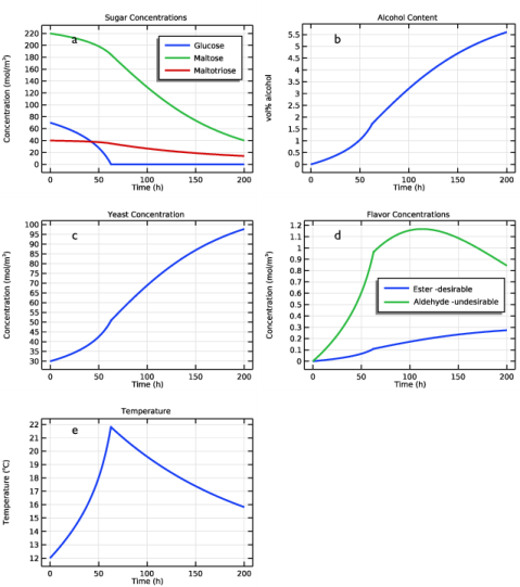
In the Settings window for Global, click Replace Expression in the upper-right corner of the y-Axis Data section. From the menu, choose Component 1 (comp1)>Reaction Engineering>re.c_G - Concentration - mol/m³.
|
|
3
|
Click Add Expression in the upper-right corner of the y-Axis Data section. From the menu, choose Component 1 (comp1)>Reaction Engineering>re.c_M - Concentration - mol/m³.
|
|
4
|
Click Add Expression in the upper-right corner of the y-Axis Data section. From the menu, choose Component 1 (comp1)>Reaction Engineering>re.c_N - Concentration - mol/m³.
|
|
5
|
|
6
|
|
7
|
|
8
|
|
10
|
|
1
|
|
2
|
|
3
|
|
4
|
In the associated text field, type vol% alcohol.
|
|
1
|
|
2
|
In the Settings window for Global, click Replace Expression in the upper-right corner of the y-Axis Data section. From the menu, choose Component 1 (comp1)>Definitions>Variables>Evol - vol% alcohol.
|
|
3
|
|
4
|
|
5
|
|
1
|
|
2
|
|
3
|
Locate the Plot Settings section. In the y-axis label text field, type Concentration (mol/m<sup>3</sup>).
|
|
1
|
|
2
|
In the Settings window for Global, click Replace Expression in the upper-right corner of the y-Axis Data section. From the menu, choose Component 1 (comp1)>Reaction Engineering>re.c_X - Concentration - mol/m³.
|
|
3
|
|
4
|
|
1
|
|
2
|
|
3
|
|
1
|
|
2
|
In the Settings window for Global, click Replace Expression in the upper-right corner of the y-Axis Data section. From the menu, choose Component 1 (comp1)>Reaction Engineering>re.c_EtAc - Concentration - mol/m³.
|
|
3
|
Click Add Expression in the upper-right corner of the y-Axis Data section. From the menu, choose Component 1 (comp1)>Reaction Engineering>re.c_AcA - Concentration - mol/m³.
|
|
4
|
|
5
|
Locate the Legends section. In the table, enter the following settings:
|
|
6
|
|
1
|
|
2
|
|
3
|
|
4
|
In the associated text field, type Temperature (<sup>o</sup>C).
|
|
1
|
|
2
|
|
4
|
|
5
|
|
6
|
|
7
|
|
8
|
|
1
|
|
2
|
|
3
|
|
4
|
Locate the Physics Interfaces section. Find the Fluid flow subsection. From the list, choose Laminar Flow: New.
|
|
5
|
|
6
|
|
7
|
|
1
|
|
2
|
|
3
|
|
4
|
Click Import.
|
|
1
|
|
2
|
In the tree, select Built-in>Air.
|
|
3
|
|
4
|
|
5
|
|
1
|
|
2
|
|
1
|
|
2
|
In the tree, select Built-in>Copper.
|
|
3
|
|
4
|
|
1
|
|
2
|
|
1
|
In the Model Builder window, under Component 2 (comp2) right-click Definitions and choose Variables.
|
|
2
|
|
3
|
|
4
|
Browse to the model’s Application Libraries folder and double-click the file beer_fermentation_variables2.txt.
|
|
1
|
|
2
|
|
3
|
|
1
|
|
2
|
|
3
|
|
1
|
|
2
|
|
3
|
|
1
|
|
2
|
|
3
|
|
1
|
|
2
|
|
3
|
|
1
|
|
2
|
|
3
|
|
1
|
|
2
|
|
3
|
|
1
|
|
2
|
|
3
|
|
1
|
|
2
|
|
3
|
|
1
|
|
2
|
|
3
|
|
1
|
In the Model Builder window, expand the Transport of Diluted Species (tds) node, then click Component 2 (comp2)>Heat Transfer in Fluids 1 (ht).
|
|
2
|
|
3
|
|
1
|
In the Model Builder window, under Component 2 (comp2)>Heat Transfer in Fluids 1 (ht) click Heat Source 1.
|
|
2
|
|
3
|
|
1
|
|
2
|
|
3
|
|
1
|
|
2
|
|
3
|
|
4
|
Locate the Model Input section. Click Make All Model Inputs Editable in the upper-right corner of the section.
|
|
5
|
|
6
|
|
1
|
|
3
|
|
4
|
|
5
|
|
6
|
|
7
|
|
1
|
|
2
|
|
3
|
|
4
|
|
1
|
|
2
|
|
3
|
|
1
|
|
1
|
|
1
|
|
2
|
|
3
|
|
4
|
|
5
|
Locate the Physics and Variables Selection section. In the table, clear the Solve for check boxes for Chemistry 1 (chem) and Transport of Diluted Species (tds).
|
|
1
|
|
1
|
|
2
|
|
3
|
In the table, select the Solve for check boxes for Chemistry 1 (chem) and Transport of Diluted Species (tds).
|
|
1
|
In the Model Builder window, expand the Study 2>Solver Configurations>Solution 2 (sol2)>Dependent Variables 1 node, then click Concentration (comp2.cAcA).
|
|
2
|
|
3
|
|
4
|
|
5
|
|
6
|
|
7
|
|
8
|
|
9
|
|
10
|
|
11
|
|
12
|
|
13
|
|
14
|
|
15
|
|
16
|
|
17
|
|
18
|
|
19
|
|
20
|
|
21
|
|
22
|
|
23
|
|
24
|
|
25
|
|
26
|
|
27
|
|
28
|
|
1
|
|
2
|
|
3
|
|
1
|
|
2
|
|
3
|
|
4
|
|
1
|
In the Model Builder window, under Results>Datasets right-click Revolution 2D 1 and choose Duplicate.
|
|
2
|
|
3
|
|
1
|
Right-click and choose Duplicate.
|
|
2
|
|
1
|
In the Model Builder window, expand the Results>Datasets>Study 2/Tank (sol2) node, then click Selection.
|
|
2
|
|
3
|
|
1
|
|
2
|
|
3
|
|
1
|
|
2
|
|
3
|
|
4
|
|
5
|
|
6
|
|
7
|
|
8
|
|
1
|
|
2
|
|
3
|
|
4
|
|
1
|
|
2
|
|
3
|
|
4
|
|
5
|
|
6
|
|
7
|
Click Define custom colors.
|
|
9
|
Click Add to custom colors.
|
|
10
|
|
11
|
|
12
|
|
13
|
Click Define custom colors.
|
|
15
|
Click Add to custom colors.
|
|
16
|
|
1
|
|
2
|
|
3
|
|
1
|
|
2
|
|
3
|
|
1
|
|
2
|
|
3
|
|
4
|
|
5
|
|
7
|
|
1
|
|
2
|
|
3
|
|
4
|
|
5
|
|
1
|
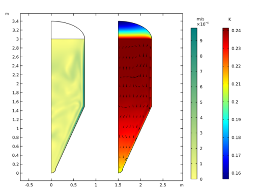
In the Settings window for Arrow Surface, click Replace Expression in the upper-right corner of the Expression section. From the menu, choose Component 2 (comp2)>Heat Transfer in Fluids 1>Domain fluxes>ht.tefluxr,ht.tefluxz - Total energy flux.
|
|
2
|
Locate the Arrow Positioning section. Find the r grid points subsection. In the Points text field, type 10.
|
|
3
|
|
4
|
|
5
|
|
6
|
|
1
|
|
2
|
|
3
|
|
4
|
|
5
|
|
1
|
|
2
|
|
3
|
|
4
|
|
5
|
|
1
|
|
2
|
In the Settings window for 2D Plot Group, type Velocity Field and Temperature in the Label text field.
|
|
1
|
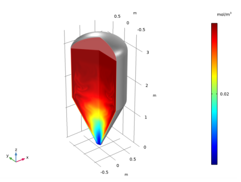
In the Model Builder window, expand the Results>Concentration, AcA, 3D (tds) node, then click Concentration, AcA, 3D (tds).
|
|
2
|
|
3
|
|
1
|
In the Model Builder window, under Results>Concentration, AcA, 3D (tds) right-click Surface 1 and choose Duplicate.
|
|
2
|
|
3
|
|
4
|
|
5
|
|
6
|
|
1
|
|
2
|
In the Settings window for 3D Plot Group, type Concentration, AcA (Acetaldehyde) in the Label text field.
|
|
1
|
|
2
|
|
3
|
|
1
|
|
2
|
|
3
|
|
1
|
|
2
|
|
3
|
|
4
|
|
5
|
|
6
|
|
1
|
|
2
|
|
3
|
|
4
|
Click Replace Expression in the upper-right corner of the Expression section. From the menu, choose Component 2 (comp2)>Heat Transfer in Fluids 1>Domain fluxes>ht.tefluxr,...,ht.tefluxz - Total energy flux.
|
|
5
|
|
6
|
|
1
|
|
2
|
|
3
|
|
1
|
|
2
|
|
1
|
|
2
|
|
1
|
|
1
|
|
2
|
|
3
|
|
1
|
|
2
|
|
3
|
|
5
|
|
6
|
|
7
|
|
8
|
|
9
|
Clear the Point check box.
|
|
10
|
|
1
|
|
2
|
|
3
|
|
4
|
|
5
|
|
7
|
|
8
|
|
1
|
|
2
|
|
3
|
Select the Plot check box.
|
|
4
|
|
5
|
|
6
|
|
1
|
|
2
|
|
3
|
|
1
|
|
2
|
|
3
|
|
4
|
|
1
|
|
2
|
|
3
|
|
4
|
|
1
|
|
2
|
|
3
|
|
1
|
|
2
|
|
3
|
|
1
|
|
2
|
|
3
|
|
1
|
|
2
|
|
3
|
|
4
|
|
1
|
|
2
|
|
3
|