PDF

Solar Panel in Periodic Flow
Introduction
This example is a study of a solar panel structure placed in a periodic flow field. The solar panel in question is located inside a regularly spaced array of panels subjected to an oncoming strong wind; see Figure 1. The model solves for the flow around the panel and the structural displacement due to the fluid load. It is assumed that enough panels are positioned both upstream and downstream of the panel for periodic flow conditions to be applicable in the streamwise direction. Seen from a position high above the ground, the array of solar panels acts as a rough boundary for the atmospheric flow.
Note: This application requires the CFD Module and the Structural Mechanics Module.
Figure 1: The modeled solar panel (in red) located in a regular array of identical panels.
Model Definition
The current investigation consists of two main parts:
Model Geometry
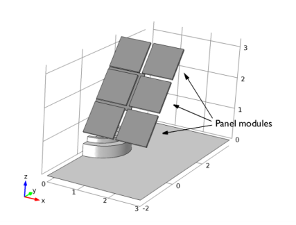
This model uses the same geometry for both the fluid-flow modeling and the subsequent structural-mechanics simulation. Figure 2 and Figure 3 show the solar panel geometry. More specifically, Figure 2 shows the solar panel’s front, which faces the flow, while Figure 3 shows its rear..
Figure 2: Front view of the solar panel geometry.
Figure 3: Rear view of the solar panel geometry.
Solution Strategy
The model uses two different studies: one solving for the turbulent flow around the solar panel using a Turbulent Flow, k-ε physics interface, and the other solving for the structural stresses and displacements using a Solid Mechanics physics interface. The Multiphysics coupling feature Fluid-Structure Interaction, Fixed Geometry, is used to couple the fluid flow boundary load from the fluid domains to the solid domains. This corresponds to a one-way fluid-structure interaction analysis.
Fluid-Flow Simulation
In the fluid-flow part, the goal is to simulate the conditions when the free-stream flow above the solar panel is about 25 m/s. This corresponds to 10 on the Beaufort scale and the land conditions “trees broken or uprooted; considerable structure damage” (Ref. 1). The Reynolds number, based on the height of the panel structure and the free stream velocity, is about 6.6·106. These conditions generate a very complex flow field. To reach a converged flow solution, the following modeling steps are applied:
1
The fluid-flow geometry is defined tall enough to capture a boundary layer type flow reaching above the array of solar panels; see Figure 4. A mapped mesh is used in the solar panels, and the fluid domain is refined to resolve the flow field. The definition of the geometry and the mesh are very important for this model, but they are rather long and complex. They are imported from the MPHBIN-file solar_panel.mphbin included in the model’s Application Libraries folder. This file was obtained from the template MPH-file solar_panel_geom.mph, also included in the model’s Application Libraries folder. The step-by-step instructions for the geometry and mesh can be found in the documentation of the Solar Panel in Periodic Flow Template model.
2
A periodic flow condition is used to prescribe a pressure difference in the streamwise direction that ensures an average velocity of 25 m/s at the top. An ODE is used to compute the pressure drop necessary to obtain the desired free stream velocity. The top boundary is modeled with a boundary stress condition.
3
Convergence in the first iterations of the nonlinear solver is ensured adding isotropic diffusion inversely proportional to the CFL number used for pseudo-time stepping. The CFL number starts at a low value (often 3 or 5), and increases as the solution progress until it reaches CFL>1000. The isotropic diffusion will have an important effect on the first iterations of the nonlinear solver, but will tend to zero as the CFL parameter increases. This strategy provides convergence without polluting the solution.
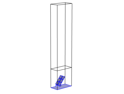
Figure 4: Computational box used in the fluid-flow simulation.
Fluid-Flow Boundary Conditions
Streamwise Conditions
A periodic flow condition is applied in the streamwise directions with a prescribed pressure difference.
Lateral Conditions
The solar panel structure is assumed to be symmetric about a streamwise plane through the center of the structure. Because identical solar panels are positioned on both sides of the panel in a regular pattern, you only need to include one half of the geometry and apply symmetry boundary conditions in the lateral directions.
Top Boundary Condition
You can apply normal stress conditions for the momentum equations to prescribe a flow of a boundary layer type at the top. Assuming that the viscous stresses are small at this position, the stress can be prescribed in accordance with a pressure decreasing linearly from the inlet to the outlet.
Structural-Mechanics Simulation
In the structural mechanics simulation, the fluid load computed from the fluid-flow simulation is applied to the solar panel structure, and then the model is solved for the resulting structural stresses and displacements. The Multiphysics coupling feature Fluid-Structure Interaction, Fixed Geometry, is used to couple the total fluid stress on the panel surfaces from the flow simulation to the structural one. Safety subnodes are added to check the risk of failure of the different materials conforming the solar panel.
Solar Panel Material
The solar panel supports — the main cylindrical base and the thinner solid supports — are made of structural steel, as is the plate on the back of the panel connecting the panel modules. The square cross-sectional bars connecting the panel modules are made of aluminum. Concerning the design of solar panels, the panel modules consist of assemblies of small solar cells. These are typically covered with glass and mounted in an aluminum frame. For simplicity, model the individual solar panel modules as made of a material with a stiffness of 3.5 GPa (5 percent the stiffness of solid aluminum), and a Poisson’s ratio of 0.33.
Structural Mechanics Boundary Conditions
The panel supports are assumed to be fixed at the ground, so that fixed constraints apply at these positions. A symmetry condition is applied to the plane where the structure has been cut in half. On the panel boundaries subjected to flow in the fluid-flow simulation, boundary loads defined from the computed total stresses are imposed.
Check the Risk of Failure
Two Safety subnodes are added to set up variables which can be used to check the risk of failure according to various criteria: Von Mises for the ductile materials (aluminum and structural steel), and Rankine for the glass. The tensile strengths of the aluminum, structural steel, and glass are assumed to be 270 MPa, 250 MPa, and 45 MPa, respectively. For the sake of security, the compressive strength of the glass is assumed to be equal to its tensile strength.
Results and Discussion
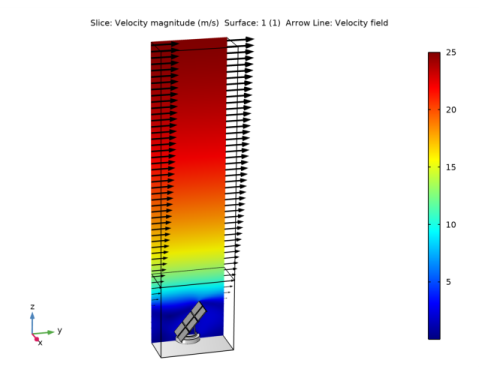
Figure 5 shows the flow-field solution around the solar panel. The figure shows the flow field in the center plane of the solar panel using a surface plot combined with velocity vectors at the inlet and outlet. The flow field above the panel is of boundary layer type with a maximum velocity of 25 m/s in the free stream. The velocity magnitude in the vicinity of the solar panel is also significantly lower due to shielding from the panels positioned upstream and downstream. The flow field can therefore be said to correspond to a rough wall turbulent boundary layer, where the solar panels act as roughness elements.
Figure 5: Final flow field in the center plane of the solar panel.
Figure 6 shows the pressure on the solar panel structure due to the surrounding flow. The maximum relative pressure, about 70 Pa, occurs in the panel’s upper-right corner. By also plotting the in-plane velocity components in a plane perpendicular to the flow direction, it is possible to find the reason for the pressure maximum at the upper-right corner. A large streamwise vortex is generated behind the panel, the center of which is aligned with the panel’s outer side. At the upper-right corner, the high pressure correlates with a high degree of deflection of the flow and formation of the streamwise vortex.
Figure 6: Surface fluid pressure contours present and in-plane velocity components 6 cm behind the panel.
The flow around the solar panel is examined in Figure 7, which shows streamlines originating at the inlet. Note that some streamlines near the center of the solar panel enter the domain and then turn around and exit, indicating that a circulation zone is present between the panels in the array. The streamlines are colored using the local turbulent kinetic energy, normalized by the kinetic energy in the free stream. The kinetic energy is low in the circulation zone in front and in the flow wake behind the panel. This is as expected because they are part of the same flow structure. The turbulent kinetic energy increases with the distance from the ground, especially when the flow passes the top of the panel. The high kinetic energy at this position correlates with a large gradient of the streamwise mean-flow velocity, as can be seen in Figure 5.
Figure 8 shows the resulting displacement of the detailed structure, and the velocity streamlines around the whole panel. In correspondence with the pressure plot in Figure 6, the largest displacement occurs in the upper-right corner. However, the maximum displacement is small, about 1 mm. This indicates that the surrounding solar panels effectively shield the solar panel from oncoming flow. It also points in the direction that for a solar panel positioned inside a large array, the fluid load on the structure at the current free stream velocity is not significant enough to dictate the design of the structure. This conclusion is supported by the minimum safety factor obtained, which is much larger than one.
Figure 7: Velocity streamlines, colored by the turbulent kinetic energy normalized by the kinetic energy in the free stream, and in-plane velocity components 6 cm behind the panel.
Figure 8: Structural displacement of the solar panel due to the fluid-flow load, and velocity streamlines colored by the velocity magnitude.
Reference
1. http://en.wikipedia.org/wiki/Beaufort_scale
Application Library path: CFD_Module/Fluid-Structure_Interaction/solar_panel
Modeling Instructions
From the File menu, choose New.
New
In the New window, click  Model Wizard.
Model Wizard
1
In the Model Wizard window, click  3D.
2
In the Select Physics tree, select Fluid Flow>Single-Phase Flow>Turbulent Flow>Turbulent Flow, k-ε (spf).
3
Click Add.
4
Click  Study.
5
In the Select Study tree, select General Studies>Stationary.
6
Global Definitions
Parameters 1
1
In the Model Builder window, under Global Definitions click Parameters 1.
2
In the Settings window for Parameters, locate the Parameters section.
3
Import the geometry and mesh.
Mesh 1
Import 1
1
In the Mesh toolbar, click  Import.
2
In the Settings window for Import, locate the Import section.
3
Click Browse.
4
5
Click Import.
Add Material
1
In the Home toolbar, click  Add Material to open the Add Material window.
2
Go to the Add Material window.
3
4
Click Add to Component in the window toolbar.
5
In the Home toolbar, click  Add Material to close the Add Material window.
Definitions
Add a nonlocal coupling that can calculate averages on the top surface.
Average 1 (aveop1)
1
In the Definitions toolbar, click  Nonlocal Couplings and choose Average.
2
In the Settings window for Average, locate the Source Selection section.
3
From the Geometric entity level list, choose Boundary.
4
Turbulent Flow, k-ε (spf)
1
In the Model Builder window, under Component 1 (comp1) click Turbulent Flow, k-ε (spf).
2
Add isotropic diffusion to improve convergence. Specify the coefficient to be inversely proportional to the pseudo time-stepping parameter CFLCMP so that the isotropic diffusion added tends to zero when CFLCMP increases.
3
Click the  Show More Options button in the Model Builder toolbar.
4
In the Show More Options dialog box, in the tree, select the check box for the node Physics>Stabilization.
5
6
In the Settings window for Turbulent Flow, k-ε, click to expand the Inconsistent Stabilization section.
7
Find the Navier-Stokes equations subsection. Select the Isotropic diffusion check box.
8
In the δid text field, type 0.5/CFLCMP.
Prescribe an approximate streamwise velocity profile and a streamwise pressure drop to go with it.
Initial Values 1
1
In the Model Builder window, expand the Turbulent Flow, k-ε (spf) node, then click Initial Values 1.
2
In the Settings window for Initial Values, locate the Initial Values section.
3
Specify the u vector as
4
In the p text field, type 0.5[Pa]*(yEnd-y)/yLen.
Periodic Flow Condition 1
1
In the Physics toolbar, click  Boundaries and choose Periodic Flow Condition.
2
3
In the Settings window for Periodic Flow Condition, locate the Pressure Difference section.
4
In the Δp text field, type pdiff.
Symmetry 1
1
In the Physics toolbar, click  Boundaries and choose Symmetry.
2
Open Boundary 1
1
In the Physics toolbar, click  Boundaries and choose Open Boundary.
2
3
In the Settings window for Open Boundary, locate the Boundary Condition section.
4
In the f0 text field, type pdiff*(yEnd-y)/yLen.
5
Locate the Turbulence Conditions section. In the Uref text field, type spf.U.
Add an ODE that calculates the pressure drop necessary to obtain a free stream velocity of 25 m/s.
6
Click the  Show More Options button in the Model Builder toolbar.
7
In the Show More Options dialog box, in the tree, select the check box for the node Physics>Equation-Based Contributions.
8
Global Equations 1
1
In the Physics toolbar, click  Global and choose Global Equations.
2
In the Settings window for Global Equations, locate the Global Equations section.
3
4
Locate the Units section. Click  Select Dependent Variable Quantity.
5
In the Physical Quantity dialog box, type pressure in the text field.
6
Click  Filter.
7
In the tree, select General>Pressure (Pa).
8
9
In the Settings window for Global Equations, locate the Units section.
10
Click  Select Source Term Quantity.
11
In the Physical Quantity dialog box, type velocity in the text field.
12
Click  Filter.
13
In the tree, select General>Velocity (m/s).
14
Study 1
Solution 1 (sol1)
1
In the Study toolbar, click  Show Default Solver.
2
In the Model Builder window, expand the Solution 1 (sol1) node.
3
In the Model Builder window, expand the Study 1>Solver Configurations>Solution 1 (sol1)>Stationary Solver 1>AMG, fluid flow variables (spf)>Multigrid 1 node.
The equation for the pressure difference is a DAE, that is, its system matrix has zeros on the diagonal and must therefore be treated with a Vanka-smoother in the iterative solver. This is already taken care of when working with the default solver for fluid flow.
4
In the Model Builder window, right-click Solution 1 (sol1) and choose Compute.
Before working with plots, disable plot when selected (Automatic update of plots). Due to the size of the datasets created, it is more convenient to generate plots actively.
Results
1
In the Settings window for Results, locate the Update of Results section.
2
Select the Only plot when requested check box.
Check the wall resolution to see if the wall distance is such that the computational domain is in the logarithmic layer.
Wall Resolution (spf)
1
In the Model Builder window, under Results click Wall Resolution (spf).
2
In the Wall Resolution (spf) toolbar, click  Plot.
The maximum wall resolution in viscous units is around 160. Since the Reynolds number is approximately 6.6·106, the wall distance is within the logarithmic layer.
To plot Figure 5 and inspect the velocity field follow the steps below.
Study 1/Solution 1 (2) (sol1)
1
In the Model Builder window, expand the Results>Datasets node.
2
Right-click Datasets and choose Solution.
Selection
1
In the Results toolbar, click  Attributes and choose Selection.
2
In the Settings window for Selection, locate the Geometric Entity Selection section.
3
From the Geometric entity level list, choose Edge.
4
Slice
1
In the Model Builder window, expand the Results>Velocity (spf) node, then click Slice.
2
In the Settings window for Slice, locate the Plane Data section.
3
From the Entry method list, choose Coordinates.
4
In the x-coordinates text field, type 1e-3.
Surface 1
1
In the Model Builder window, right-click Velocity (spf) and choose Surface.
2
In the Settings window for Surface, locate the Data section.
3
From the Dataset list, choose Exterior Walls.
4
Locate the Expression section. In the Expression text field, type 1.
5
Locate the Coloring and Style section. From the Coloring list, choose Uniform.
6
From the Color list, choose Gray.
Arrow Line 1
1
Right-click Velocity (spf) and choose Arrow Line.
2
In the Settings window for Arrow Line, locate the Data section.
3
From the Dataset list, choose Study 1/Solution 1 (2) (sol1).
4
Locate the Coloring and Style section. Select the Scale factor check box.
5
6
Locate the Arrow Positioning section. In the Number of arrows text field, type 100.
7
Locate the Coloring and Style section. From the Color list, choose Black.
8
In the Velocity (spf) toolbar, click  Plot.
To plot the pressure as done in Figure 6 perform the following steps
Cut Plane 1
1
In the Results toolbar, click  Cut Plane.
2
In the Settings window for Cut Plane, locate the Data section.
3
From the Dataset list, choose Study 1/Solution 1 (2) (sol1).
4
Locate the Plane Data section. From the Plane list, choose zx-planes.
5
In the y-coordinate text field, type 2.0.
Pressure
1
In the Model Builder window, expand the Results>Pressure (spf) node.
2
Right-click Pressure and choose Delete.
Pressure (spf)
In the Model Builder window, click Pressure (spf).
Surface 2
1
In the Pressure (spf) toolbar, click  Surface.
2
In the Settings window for Surface, locate the Expression section.
3
In the Expression text field, type p.
Arrow Surface 1
1
Right-click Pressure (spf) and choose Arrow Surface.
2
In the Settings window for Arrow Surface, locate the Data section.
3
From the Dataset list, choose Cut Plane 1.
4
Locate the Expression section. In the y component text field, type 0.
5
Locate the Coloring and Style section. From the Color list, choose Black.
6
Locate the Arrow Positioning section. In the Number of arrows text field, type 800.
7
In the Pressure (spf) toolbar, click  Plot.
Follow the steps below to create Figure 7, which plots fluid flow streamlines colored by the turbulent kinetic energy.
Streamline plot
1
Right-click Pressure (spf) and choose Duplicate.
2
Right-click Pressure (spf) 1 and choose Rename.
3
In the Rename 3D Plot Group dialog box, type Streamline plot in the New label text field.
4
Surface 2
1
In the Model Builder window, expand the Streamline plot node.
2
Right-click Surface 2 and choose Delete.
Streamline plot
1
In the Model Builder window, click Streamline plot.
2
Click Yes to confirm.
Streamline 1
1
Right-click Streamline plot and choose Streamline.
2
In the Settings window for Streamline, locate the Data section.
3
From the Dataset list, choose Study 1/Solution 1 (2) (sol1).
4
Locate the Streamline Positioning section. From the Entry method list, choose Coordinates.
5
In the x text field, type 0.5*1^range(1,7), 1.0*1^range(1,7), 1.75*1^range(1,7).
6
In the y text field, type -2.
7
In the z text field, type range(0.5,3/6,3.5), range(0.5,3/6,3.5), range(0.5,3/6,3.5).
8
Locate the Coloring and Style section. Find the Line style subsection. From the Type list, choose Ribbon.
9
Select the Width scale factor check box.
10
Color Expression 1
1
Right-click Streamline 1 and choose Color Expression.
2
In the Settings window for Color Expression, locate the Expression section.
3
In the Expression text field, type k/(0.5*25^2).
4
Locate the Coloring and Style section. From the Color table list, choose WaveLight.
5
In the Streamline plot toolbar, click  Plot.
This concludes the study of the flow field. The next step is to add the structural analysis and couple it with the flow field.
Add new selections to be used when setting up the Solid Mechanics physics interface and in the plots.
Definitions
Walls
1
In the Definitions toolbar, click  Explicit.
2
In the Settings window for Explicit, type Walls in the Label text field.
3
Locate the Input Entities section. From the Geometric entity level list, choose Boundary.
4
Click  Paste Selection.
5
In the Paste Selection dialog box, type 3 9 10 11 14 17 18 19 22 23 24 25 26 27 28 30 31 33 34 35 38 41 42 43 45 46 47 53 54 55 57 60 63 66 69 99 100 101 102 104 105 106 112 113 114 116 117 120 121 122 123 127 128 130 131 132 133 141 142 143 146 147 148 150 152 153 154 156 157 159 160 161 163 164 166 167 168 169 170 171 172 173 174 176 177 179 180 181 183 184 185 187 189 192 194 195 196 197 198 200 202 203 204 205 206 207 208 209 210 211 212 214 215 216 218 219 222 223 224 225 226 229 231 234 235 236 241 242 245 246 247 248 249 254 257 258 259 263 264 265 267 268 270 271 272 273 274 276 277 278 279 280 281 282 284 285 286 287 288 289 290 292 293 294 295 296 297 298 300 301 302 303 304 305 307 308 309 310 311 312 313 314 315 316 317 318 in the Selection text field.
6
Supports
1
In the Definitions toolbar, click  Explicit.
2
In the Settings window for Explicit, type Supports in the Label text field.
3
Locate the Input Entities section. From the Geometric entity level list, choose Boundary.
4
Click  Paste Selection.
5
In the Paste Selection dialog box, type 29 58 93 175 182 in the Selection text field.
6
Symmetry
1
In the Definitions toolbar, click  Explicit.
2
In the Settings window for Explicit, type Symmetry in the Label text field.
3
Locate the Input Entities section. From the Geometric entity level list, choose Boundary.
4
Click  Paste Selection.
5
In the Paste Selection dialog box, type 8 12 15 20 32 36 39 44 48 51 56 59 62 65 68 78 81 84 91 95 103 107 110 115 118 124 129 in the Selection text field.
6
Structural steel
1
In the Definitions toolbar, click  Explicit.
2
In the Settings window for Explicit, type Structural steel in the Label text field.
3
Locate the Input Entities section. Click  Paste Selection.
4
In the Paste Selection dialog box, type 4 5 6 8 9 11 12 13 14 15 16 17 21 22 24 25 27 33 34 35 40 42 45 47 in the Selection text field.
5
Aluminum
1
In the Definitions toolbar, click  Explicit.
2
In the Settings window for Explicit, type Aluminum in the Label text field.
3
Locate the Input Entities section. Click  Paste Selection.
4
In the Paste Selection dialog box, type 3 7 10 18 19 20 23 26 28 30 36 38 41 43 46 in the Selection text field.
5
Glass
1
In the Definitions toolbar, click  Explicit.
2
In the Settings window for Explicit, type Glass in the Label text field.
3
Locate the Input Entities section. Click  Paste Selection.
4
In the Paste Selection dialog box, type 29 31 32 37 39 44 in the Selection text field.
5
Solid Domains
1
In the Definitions toolbar, click  Union.
2
In the Settings window for Union, type Solid Domains in the Label text field.
3
Locate the Input Entities section. Under Selections to add, click  Add.
4
In the Add dialog box, in the Selections to add list, choose Structural steel, Aluminum, and Glass.
5
Solid Domains except Glass
1
In the Definitions toolbar, click  Union.
2
In the Settings window for Union, type Solid Domains except Glass in the Label text field.
3
Locate the Input Entities section. Under Selections to add, click  Add.
4
In the Add dialog box, in the Selections to add list, choose Structural steel and Aluminum.
5
Exterior Boundaries to Solid Domains
1
In the Definitions toolbar, click  Adjacent.
2
In the Settings window for Adjacent, type Exterior Boundaries to Solid Domains in the Label text field.
3
Locate the Input Entities section. Under Input selections, click  Add.
4
In the Add dialog box, select Solid Domains in the Input selections list.
5
Floor and Solar Panel Base
1
In the Definitions toolbar, click  Difference.
2
In the Settings window for Difference, type Floor and Solar Panel Base in the Label text field.
3
Locate the Geometric Entity Level section. From the Level list, choose Boundary.
4
Locate the Input Entities section. Under Selections to add, click  Add.
5
In the Add dialog box, select Walls in the Selections to add list.
6
7
In the Settings window for Difference, locate the Input Entities section.
8
Under Selections to subtract, click  Add.
9
In the Add dialog box, select Exterior Boundaries to Solid Domains in the Selections to subtract list.
10
Add Physics
1
In the Home toolbar, click  Add Physics to open the Add Physics window.
2
Go to the Add Physics window.
3
In the tree, select Structural Mechanics>Solid Mechanics (solid).
4
Click Add to Component 1 in the window toolbar.
5
In the Home toolbar, click  Add Physics to close the Add Physics window.
Solid Mechanics (solid)
1
In the Settings window for Solid Mechanics, locate the Domain Selection section.
2
From the Selection list, choose Solid Domains.
Linear Elastic Material 1
In the Model Builder window, under Component 1 (comp1)>Solid Mechanics (solid) click Linear Elastic Material 1.
Safety 1
1
In the Physics toolbar, click  Attributes and choose Safety.
2
In the Settings window for Safety, locate the Domain Selection section.
3
From the Selection list, choose Solid Domains except Glass.
Linear Elastic Material 1
In the Model Builder window, click Linear Elastic Material 1.
Safety 2
1
In the Physics toolbar, click  Attributes and choose Safety.
2
In the Settings window for Safety, locate the Domain Selection section.
3
From the Selection list, choose Glass.
4
Locate the Failure Model section. From the Failure criterion list, choose Rankine.
Add Multiphysics
1
In the Physics toolbar, click  Add Multiphysics to open the Add Multiphysics window.
2
Go to the Add Multiphysics window.
3
In the tree, select Fluid Flow>Fluid-Structure Interaction>Fluid-Solid Interaction, Fixed Geometry.
4
Click Add to Component in the window toolbar.
5
In the Physics toolbar, click  Add Multiphysics to close the Add Multiphysics window.
Multiphysics
Fluid-Structure Interaction 1 (fsi1)
1
In the Settings window for Fluid-Structure Interaction, locate the Fixed Geometry section.
2
From the Fixed geometry coupling type list, choose Fluid loading on structure.
Add Material
1
In the Home toolbar, click  Add Material to open the Add Material window.
2
Go to the Add Material window.
3
In the tree, select Built-in>Structural steel.
4
Click Add to Component in the window toolbar.
5
In the tree, select Built-in>Aluminum.
6
Click Add to Component in the window toolbar.
7
In the Home toolbar, click  Add Material to close the Add Material window.
Materials
Air (mat1)
1
In the Model Builder window, under Component 1 (comp1)>Materials click Air (mat1).
2
In the Settings window for Material, locate the Geometric Entity Selection section.
3
From the Selection list, choose Manual.
4
Click  Clear Selection.
5
Structural steel (mat2)
1
In the Model Builder window, click Structural steel (mat2).
2
In the Settings window for Material, locate the Geometric Entity Selection section.
3
From the Selection list, choose Structural steel.
4
Locate the Material Contents section. In the table, enter the following settings:
Aluminum (mat3)
1
In the Model Builder window, click Aluminum (mat3).
2
In the Settings window for Material, locate the Geometric Entity Selection section.
3
From the Selection list, choose Aluminum.
4
Locate the Material Contents section. In the table, enter the following settings:
Glass
1
In the Model Builder window, right-click Materials and choose Blank Material.
2
In the Settings window for Material, type Glass in the Label text field.
3
Locate the Geometric Entity Selection section. From the Selection list, choose Glass.
4
Locate the Material Contents section. In the table, enter the following settings:
Solid Mechanics (solid)
Fixed Constraint 1
1
In the Physics toolbar, click  Boundaries and choose Fixed Constraint.
2
In the Settings window for Fixed Constraint, locate the Boundary Selection section.
3
From the Selection list, choose Supports.
Symmetry 1
1
In the Physics toolbar, click  Boundaries and choose Symmetry.
2
In the Settings window for Symmetry, locate the Boundary Selection section.
3
From the Selection list, choose Symmetry.
Add Study
1
In the Home toolbar, click  Add Study to open the Add Study window.
2
Go to the Add Study window.
3
Find the Studies subsection. In the Select Study tree, select General Studies>Stationary.
4
Click Add Study in the window toolbar.
5
In the Home toolbar, click  Add Study to close the Add Study window.
Study 2
1
In the Model Builder window, click Study 2.
2
In the Settings window for Study, locate the Study Settings section.
3
Clear the Generate default plots check box.
Step 1: Stationary
1
In the Model Builder window, under Study 2 click Step 1: Stationary.
2
In the Settings window for Stationary, locate the Physics and Variables Selection section.
3
In the table, clear the Solve for check box for Turbulent Flow, k-ε (spf).
4
Click to expand the Values of Dependent Variables section. Find the Values of variables not solved for subsection. From the Settings list, choose User controlled.
5
From the Method list, choose Solution.
6
From the Study list, choose Study 1, Stationary.
Use an iterative solver to reduce the memory requirements.
Solution 2 (sol2)
1
In the Study toolbar, click  Show Default Solver.
2
In the Model Builder window, expand the Solution 2 (sol2) node.
3
In the Model Builder window, expand the Study 2>Solver Configurations>Solution 2 (sol2)>Stationary Solver 1 node.
4
Right-click Suggested Iterative Solver (solid) and choose Enable.
5
In the Study toolbar, click  Compute.
Results
Study 2/Solution 2, Solid Domains
1
In the Results toolbar, click  More Datasets and choose Solution.
2
In the Settings window for Solution, type Study 2/Solution 2, Solid Domains in the Label text field.
3
Locate the Solution section. From the Solution list, choose Solution 2 (sol2).
Selection
1
In the Results toolbar, click  Attributes and choose Selection.
2
In the Settings window for Selection, locate the Geometric Entity Selection section.
3
From the Geometric entity level list, choose Domain.
4
From the Selection list, choose Solid Domains.
Mirror 3D, Solution 1
1
In the Results toolbar, click  More Datasets and choose Mirror 3D.
2
In the Settings window for Mirror 3D, type Mirror 3D, Solution 1 in the Label text field.
Mirror 3D, Solid Domains
1
In the Results toolbar, click  More Datasets and choose Mirror 3D.
2
In the Settings window for Mirror 3D, type Mirror 3D, Solid Domains in the Label text field.
3
Locate the Data section. From the Dataset list, choose Study 2/Solution 2, Solid Domains (sol2).
Floor and Solar Panel Base
1
In the Results toolbar, click  More Datasets and choose Surface.
2
In the Settings window for Surface, type Floor and Solar Panel Base in the Label text field.
3
Locate the Selection section. From the Selection list, choose Floor and Solar Panel Base.
Mirror 3D, Floor and Solar Panel Base
1
In the Results toolbar, click  More Datasets and choose Mirror 3D.
2
In the Settings window for Mirror 3D, type Mirror 3D, Floor and Solar Panel Base in the Label text field.
3
Locate the Data section. From the Dataset list, choose Floor and Solar Panel Base.
Stress (solid)
1
In the Results toolbar, click  3D Plot Group.
2
In the Settings window for 3D Plot Group, type Stress (solid) in the Label text field.
3
Locate the Data section. From the Dataset list, choose Study 2/Solution 2 (sol2).
Surface 1
1
Right-click Stress (solid) and choose Surface.
2
In the Settings window for Surface, locate the Expression section.
3
In the Expression text field, type solid.mises.
4
Locate the Coloring and Style section. From the Color table list, choose RainbowLight.
Deformation 1
1
Right-click Surface 1 and choose Deformation.
2
In the Stress (solid) toolbar, click  Plot.
Displacement magnitude and streamlines
1
In the Home toolbar, click  Add Plot Group and choose 3D Plot Group.
2
In the Settings window for 3D Plot Group, type Displacement magnitude and streamlines in the Label text field.
3
Locate the Plot Settings section. Clear the Plot dataset edges check box.
Surface 1
1
Right-click Displacement magnitude and streamlines and choose Surface.
2
In the Settings window for Surface, locate the Data section.
3
From the Dataset list, choose Mirror 3D, Solid Domains.
4
Click Replace Expression in the upper-right corner of the Expression section. From the menu, choose Component 1 (comp1)>Solid Mechanics>Displacement>solid.disp - Displacement magnitude - m.
5
Locate the Coloring and Style section. From the Color table list, choose JupiterAuroraBorealis.
6
Select the Reverse color table check box.
Displacement magnitude and streamlines
In the Model Builder window, click Displacement magnitude and streamlines.
Streamline 1
1
In the Displacement magnitude and streamlines toolbar, click  Streamline.
2
In the Settings window for Streamline, locate the Data section.
3
From the Dataset list, choose Mirror 3D, Solution 1.
4
Locate the Streamline Positioning section. From the Entry method list, choose Coordinates.
5
In the x text field, type -1.75*1^range(1,7), -0.5*1^range(1,7), 0.5*1^range(1,7), 1.75*1^range(1,7).
6
In the y text field, type -2.
7
In the z text field, type range(0.5,3/6,3.5), range(0.5,3/6,3.5), range(0.5,3/6,3.5), range(0.5,3/6,3.5).
8
Locate the Coloring and Style section. Find the Line style subsection. From the Type list, choose Ribbon.
9
In the Width expression text field, type 0.03.
10
Select the Width scale factor check box.
Color Expression 1
1
Right-click Streamline 1 and choose Color Expression.
2
In the Settings window for Color Expression, locate the Coloring and Style section.
3
From the Color table list, choose WaveLight.
Surface 2
1
In the Model Builder window, right-click Displacement magnitude and streamlines and choose Surface.
2
In the Settings window for Surface, locate the Data section.
3
From the Dataset list, choose Mirror 3D, Floor and Solar Panel Base.
4
Locate the Expression section. In the Expression text field, type 0.
5
Click to expand the Title section. From the Title type list, choose None.
6
Click to expand the Inherit Style section. From the Plot list, choose Surface 1.
7
In the Displacement magnitude and streamlines toolbar, click  Plot.
Plot the safety factor to check that the structure is far from failure.
3D Plot Group 7
1
In the Home toolbar, click  Add Plot Group and choose 3D Plot Group.
2
In the Settings window for 3D Plot Group, locate the Data section.
3
From the Dataset list, choose Study 2/Solution 2, Solid Domains (sol2).
4
Locate the Plot Settings section. Clear the Plot dataset edges check box.
Volume 1
1
Right-click 3D Plot Group 7 and choose Volume.
2
In the Settings window for Volume, click Replace Expression in the upper-right corner of the Expression section. From the menu, choose Component 1 (comp1)>Solid Mechanics>Safety>von Mises>solid.lemm1.sf1.s_f - von Mises safety factor.
3
Click to expand the Range section. Select the Manual color range check box.
4
In the Maximum text field, type 2000.
5
Locate the Coloring and Style section. From the Color table list, choose RainbowLight.
6
Select the Reverse color table check box.
3D Plot Group 7
In the Model Builder window, click 3D Plot Group 7.
Max/Min Volume 1
1
In the 3D Plot Group 7 toolbar, click  More Plots and choose Max/Min Volume.
2
In the Settings window for Max/Min Volume, click Replace Expression in the upper-right corner of the Expression section. From the menu, choose Component 1 (comp1)>Solid Mechanics>Safety>von Mises>solid.lemm1.sf1.s_f - von Mises safety factor.
3
Click to expand the Advanced section. Locate the Display section. From the Display list, choose Min.
4
Locate the Coloring and Style section. From the Background color list, choose White.
Safety factor, ductile materials
1
Right-click 3D Plot Group 7 and choose Rename.
2
In the Rename 3D Plot Group dialog box, type Safety factor, ductile materials in the New label text field.
3
4
In the Safety factor, ductile materials toolbar, click  Plot.
The minimum safety factor for the ductile materials (steel and aluminum) is much larger than one, and they work within the elastic regime.
3D Plot Group 8
1
In the Home toolbar, click  Add Plot Group and choose 3D Plot Group.
2
In the Settings window for 3D Plot Group, locate the Data section.
3
From the Dataset list, choose Study 2/Solution 2, Solid Domains (sol2).
4
Locate the Plot Settings section. Clear the Plot dataset edges check box.
Volume 1
1
Right-click 3D Plot Group 8 and choose Volume.
2
In the Settings window for Volume, click Replace Expression in the upper-right corner of the Expression section. From the menu, choose Component 1 (comp1)>Solid Mechanics>Safety>Rankine>solid.lemm1.sf2.s_f - Rankine safety factor.
3
Locate the Range section. Select the Manual color range check box.
4
In the Maximum text field, type 2000.
5
Locate the Coloring and Style section. From the Color table list, choose RainbowLight.
6
Select the Reverse color table check box.
3D Plot Group 8
In the Model Builder window, click 3D Plot Group 8.
Max/Min Volume 1
1
In the 3D Plot Group 8 toolbar, click  More Plots and choose Max/Min Volume.
2
In the Settings window for Max/Min Volume, click Replace Expression in the upper-right corner of the Expression section. From the menu, choose Component 1 (comp1)>Solid Mechanics>Safety>Rankine>solid.lemm1.sf2.s_f - Rankine safety factor.
3
Locate the Display section. From the Display list, choose Min.
4
Locate the Coloring and Style section. From the Background color list, choose White.
Safety factor, glass
1
Right-click 3D Plot Group 8 and choose Rename.
2
In the Rename 3D Plot Group dialog box, type Safety factor, glass in the New label text field.
3
4
In the Safety factor, glass toolbar, click  Plot.
The minimum safety factor for the glass is large enough to consider that the structure is far from failure.