PDF

Rising Bubble
Introduction
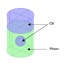
This example shows how to model two immiscible fluids, tracking the fluid-fluid interface. An oil bubble rises through water and merges with oil already residing at the top of the container. Initially three different regions exist: the initially still oil bubble, the oil at the top of the container, and the water surrounding the bubble (see Figure 1). The container is cylindrical with a diameter of 1·102 m and a height of 1.5·102 m. The oil phase has a viscosity of 0.0208 Pa·s and has a density of 879 kg/m3. For water the viscosity is 1.01·103 Pa·s and the density is 1000 kg/m3. Buoyancy effects cause the oil bubble to rise through the water phase. As the bubble reaches the liquid-liquid interface, it merges with the oil phase.
Figure 1: Initial bubble position. The geometry is axisymmetric.
As outlined above, the topology of the fluid interface changes with time. You start with three separate fluid regions and end up with two. The level set method as well as the phase field method are both well suited for modeling moving boundaries where topology changes occur. Both methods are available in the CFD Module as predefined physics interfaces. This example shows you how to use the Laminar Two-Phase Flow, Level Set interface.
Model Definition
Representation and Convection of the Fluid Interface
The Level Set interface finds the fluid interface by tracing the isolines of the level set function, . The level set or isocontour determines the position of the interface. The equation governing the transport and reinitialization of is
where u (SI unit: m/s) is the fluid velocity, and γ (SI unit: m/s) and ε (SI unit: m) are reinitialization parameters. The ε parameter determines the thickness of the layer around the interface where goes from zero to one. When stabilization is used for the level set equation, you can typically use an interface thickness of ε = hc/2, where hc is the characteristic mesh size in the region passed by the interface. The γ parameter determines the amount of reinitialization. A suitable value for γ is the maximum velocity magnitude occurring in the model.
Because the level set function is a smooth step function, it is also used to determine the density and dynamic viscosity globally by
and
Here ρw, μw, ρo, and μo denote the constant density and viscosity of water and oil, respectively.
Mass and Momentum Transport
In the Laminar Two-Phase Flow, Level Set interface, the transport of mass and momentum is governed by the incompressible Navier-Stokes equations, including surface tension:
In the above equations, ρ (SI unit: kg/m3) denotes the density, u is the velocity (SI unit: m/s), t equals time (SI unit: s), p is the pressure (SI unit: Pa), and μ denotes the viscosity (SI unit: Pa·s). The momentum equations contain gravity, ρg, and surface tension force components, denoted by Fst.
Surface Tension
The surface tension force is defined by
where σ is the surface tension coefficient, I is the identity matrix, n is the interface unit normal, and δ is a Dirac delta function, nonzero only at the fluid interface. The interface normal is calculated from
The level set parameter is also used to approximate the delta function by a smooth function defined by
Initial Condition
At t = 0, the velocity is zero. Figure 2 shows the initial level set function. This is automatically computed using a Phase Initialization study step by solving for the geometrical distance to the initial interface, Dwi. The initialized level set function is then defined from the analytical steady state solution for a straight fluid-fluid interface:
in the domains initially filled with Fluid 1 and Fluid 2 respectively,
Figure 2: A surface and contour plot of the initialized level set function.
Boundary Conditions
Use no slip conditions, u = 0 at the top and bottom and a wetted wall condition on the right boundary. The left boundary corresponds to the symmetry axis.
Results and Discussion
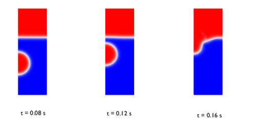
Figure 3 and Figure 4 contain snapshots of the fluid interface. The snapshots show how the bubble travels up through the water and merges with the oil above. As the bubble rises, its shape remains spherical due to the surface tension and the high viscosity of the oil. As the droplet hits the water surface, it merges with the oil above and creates waves on the surface.
Figure 3: Snapshots showing the interface prior to and just after the bubble hits the surface.
Figure 4: Snapshots showing the interface after the bubble has merged with the oil above.
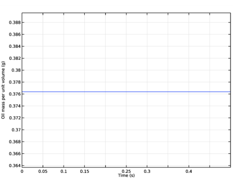
One way to investigate the quality of the numerical results is to check the conservation of mass. Because there are no reactions and no flow through the boundaries, the total mass of each fluid should be constant in time. Figure 5 shows the total mass of oil as a function of time. The mass loss during simulation is small, showing that the model conserves mass. Exact mass conservation is obtained when using the conservative level set form. However, the conservative form is less suited for numerical calculations and convergence is harder.
Figure 5: Total mass of oil as a function of time. The total mass loss during the simulation is conserved.
Notes About the COMSOL Implementation
The model is straightforward to set up and solve using either the Laminar Two-Phase Flow, Level Set interface. Automatically, two study steps are created. The first one initializes the level set function, and the second one calculates the dynamic two phase flow problem.
Application Library path: CFD_Module/Multiphase_Flow/rising_bubble_2daxi
Modeling Instructions
From the File menu, choose New.
New
In the New window, click  Model Wizard.
Model Wizard
1
In the Model Wizard window, click  2D Axisymmetric.
2
In the Select Physics tree, select Fluid Flow>Multiphase Flow>Two-Phase Flow, Level Set>Laminar Flow.
3
Click Add.
4
Click  Study.
5
In the Select Study tree, select Preset Studies for Selected Multiphysics>Time Dependent with Phase Initialization.
6
Geometry 1
1
In the Model Builder window, under Component 1 (comp1) click Geometry 1.
2
In the Settings window for Geometry, locate the Units section.
3
From the Length unit list, choose mm.
Rectangle 1 (r1)
1
In the Geometry toolbar, click  Rectangle.
2
In the Settings window for Rectangle, locate the Size and Shape section.
3
In the Width text field, type 5.
4
In the Height text field, type 15.
5
Click  Build Selected.
Polygon 1 (pol1)
1
In the Geometry toolbar, click  Polygon.
2
In the Settings window for Polygon, locate the Coordinates section.
3
From the Data source list, choose Vectors.
4
In the r text field, type 0 5.
5
In the z text field, type 10.
6
Click  Build Selected.
Circle 1 (c1)
1
In the Geometry toolbar, click  Circle.
2
In the Settings window for Circle, locate the Size and Shape section.
3
In the Radius text field, type 2.
4
In the Sector angle text field, type 180.
5
Locate the Position section. In the z text field, type 4.
6
Locate the Rotation Angle section. In the Rotation text field, type -90.
7
Click  Build Selected.
Form Union (fin)
1
In the Model Builder window, click Form Union (fin).
2
In the Settings window for Form Union/Assembly, click  Build Selected.
Add Material
1
In the Home toolbar, click  Add Material to open the Add Material window.
2
Go to the Add Material window.
3
In the tree, select Liquids and Gases>Liquids>Transformer oil.
4
Click Add to Component in the window toolbar.
5
In the tree, select Liquids and Gases>Liquids>Water.
6
Click Add to Component in the window toolbar.
7
In the Home toolbar, click  Add Material to close the Add Material window.
You can leave the Geometric Entity Selection empty at this stage; it will be defined when you use this material in the Fluid Properties feature.
Multiphysics
Two-Phase Flow, Level Set 1 (tpf1)
1
In the Model Builder window, under Component 1 (comp1)>Multiphysics click Two-Phase Flow, Level Set 1 (tpf1).
2
In the Settings window for Two-Phase Flow, Level Set, locate the Fluid 1 Properties section.
3
From the Fluid 1 list, choose Transformer oil (mat1).
4
Locate the Fluid 2 Properties section. From the Fluid 2 list, choose Water (mat2).
5
Locate the Surface Tension section. Select the Include surface tension force in momentum equation check box.
6
From the Surface tension coefficient list, choose Library coefficient, liquid/liquid interface.
7
From the list, choose Olive oil/Water, 20°C.
Level Set (ls)
Level Set Model 1
1
In the Model Builder window, under Component 1 (comp1)>Level Set (ls) click Level Set Model 1.
2
In the Settings window for Level Set Model, locate the Level Set Model section.
3
In the γ text field, type 0.2.
Initial Values, Fluid 2
1
In the Model Builder window, click Initial Values, Fluid 2.
2
Laminar Flow (spf)
1
In the Model Builder window, under Component 1 (comp1) click Laminar Flow (spf).
2
In the Settings window for Laminar Flow, locate the Physical Model section.
3
Select the Include gravity check box.
Pressure Point Constraint 1
1
In the Physics toolbar, click  Points and choose Pressure Point Constraint.
2
Multiphysics
Wetted Wall 1 (ww1)
1
In the Model Builder window, under Component 1 (comp1)>Multiphysics click Wetted Wall 1 (ww1).
2
Before creating the mesh, add a variable for computing the mass of oil in the model domain. You will use this variable later to test mass conservation.
Definitions
Variables 1
1
In the Home toolbar, click  Variables and choose Local Variables.
2
In the Settings window for Variables, locate the Variables section.
3
Mesh 1
Free Triangular 1
In the Mesh toolbar, click  Free Triangular.
Size
1
In the Model Builder window, click Size.
2
In the Settings window for Size, locate the Element Size section.
3
From the Calibrate for list, choose Fluid dynamics.
4
From the Predefined list, choose Finer.
5
Click  Build All.
Study 1
Step 2: Time Dependent
1
In the Model Builder window, under Study 1 click Step 2: Time Dependent.
2
In the Settings window for Time Dependent, locate the Study Settings section.
3
In the Output times text field, type range(0,0.5/50,0.5).
Solution 1 (sol1)
1
In the Study toolbar, click  Show Default Solver.
2
In the Settings window for Solution, click  Compute.
Results
Next, test to what degree the total mass of oil is conserved.
Surface Integration 1
1
In the Results toolbar, click  More Derived Values and choose Integration>Surface Integration.
2
In the Settings window for Surface Integration, locate the Selection section.
3
From the Selection list, choose All domains.
4
Click Replace Expression in the upper-right corner of the Expressions section. From the menu, choose Component 1 (comp1)>Definitions>Variables>rho_oil - Oil mass per unit volume - kg/m³.
5
Locate the Expressions section. In the table, enter the following settings:
6
Click  Evaluate.
Table
1
Go to the Table window.
2
Click Table Graph in the window toolbar.
Results
1D Plot Group 6
1
In the Model Builder window, under Results click 1D Plot Group 6.
2
In the Settings window for 1D Plot Group, locate the Axis section.
3
Select the Manual axis limits check box.
4
In the x minimum text field, type 0.
5
In the x maximum text field, type 0.5.
6
In the y minimum text field, type 0.3637.
7
In the y maximum text field, type 0.3896.
Compare the result to that in Figure 5. As the plot shows, mass is conserved.
Volume Fraction of Fluid 1 (ls)
1
In the Model Builder window, click Volume Fraction of Fluid 1 (ls).
2
In the Settings window for 2D Plot Group, locate the Plot Settings section.
3
Clear the Plot dataset edges check box.
Volume Fraction of Fluid 1
1
In the Model Builder window, expand the Volume Fraction of Fluid 1 (ls) node, then click Volume Fraction of Fluid 1.
2
In the Settings window for Surface, locate the Coloring and Style section.
3
From the Color table list, choose WaveLight.
Volume Fraction of Fluid 1 (ls)
To reproduce the plots in Figure 2 and Figure 3, plot the solution for the time values 0 0.08 0.12, 0.16, 0.20, 0.26, and 0.32.
1
In the Model Builder window, click Volume Fraction of Fluid 1 (ls).
2
In the Settings window for 2D Plot Group, locate the Data section.
3
From the Time (s) list, choose 0.
4
In the Volume Fraction of Fluid 1 (ls) toolbar, click  Plot.
Repeat the last two steps for the time values 0.08 0.12, 0.16, 0.20, 0.26, and 0.32 s.
Volume Fraction of Fluid 1 (ls) 1
Add a slice plot of the velocity magnitude to the axisymmetric model revolved into 3D
Slice 1
1
In the Model Builder window, expand the Results>Velocity, 3D (spf) node.
2
Right-click Volume Fraction of Fluid 1 (ls) 1 and choose Slice.
3
In the Settings window for Slice, locate the Plane Data section.
4
From the Plane list, choose zx-planes.
5
In the Planes text field, type 1.
6
Locate the Coloring and Style section. From the Color table list, choose JupiterAuroraBorealis.
Isosurface 1
1
In the Model Builder window, click Isosurface 1.
2
In the Settings window for Isosurface, locate the Coloring and Style section.
3
From the Color list, choose Black.
Volume Fraction of Fluid 1 (ls) 1
1
In the Model Builder window, click Volume Fraction of Fluid 1 (ls) 1.
2
In the Settings window for 3D Plot Group, locate the Data section.
3
From the Time (s) list, choose 0.11.
4
In the Volume Fraction of Fluid 1 (ls) 1 toolbar, click  Plot.
Edge 2D 1
1
In the Results toolbar, click  More Datasets and choose Edge 2D.
2
Revolution 2D 3
1
In the Results toolbar, click  More Datasets and choose Revolution 2D.
2
In the Settings window for Revolution 2D, locate the Data section.
3
From the Dataset list, choose Edge 2D 1.
4
Click to expand the Revolution Layers section. In the Revolution angle text field, type 180.
Surface 1
1
Right-click Volume Fraction of Fluid 1 (ls) 1 and choose Surface.
2
In the Settings window for Surface, locate the Data section.
3
From the Dataset list, choose Revolution 2D 3.
4
Locate the Coloring and Style section. From the Coloring list, choose Uniform.
5
From the Color list, choose Gray.
Finally, create a movie using the current plot group.
Animation 1
1
In the Volume Fraction of Fluid 1 (ls) 1 toolbar, click  Animation and choose Player.
2
Right-click Animation 1 and choose Play.