PDF

Phase Separation
Introduction
Phase separation occurs when a binary system is quenched from a stable, homogeneous one-phase state into the two-phase region of its phase diagram. The spontaneous separation of two immiscible fluids is sometimes referred to as spinodal decomposition. Each phase tends to separate into pure components. This example demonstrates how to use the Phase Field interface to model the process of phase separation, see Ref. 1 for more information.
Model Definition
This simple benchmark model takes two initially mixed, immiscible phases and observes their separation into pure components. The components are represented by a phase field function, , and are considered pure when . The initial mixture is created by putting equal to a random number with zero mean and a standard deviation of 0.05. The initial random perturbation initiates the separation into pure phases.
The separation of the two immiscible phases is described by the Cahn-Hilliard equation:
where is the dimensionless phase field variable, so that the volume fractions of the components of the fluid are and . The variable γ is the mobility (m3·s/kg), the quantity λ is the mixing energy density (N), and ε is a capillary width that scales with the thickness of the interface (m). The latter two parameters are related to the surface tension coefficient through the equation
The equation governing ψ is
In the Phase Field interface, the volume fractions of the individual fluids are
The Wetted Wall default boundary condition is imposed on the boundary. Mathematically, the boundary condition is
and
In COMSOL Multiphysics, the only input required is a contact angle, θw.
The total mass in the system is computed by integrating the phase field variable over the domain:
(1)
This integrated quantity should remain constant during the separation of the two phases.
Results and Discussion
Figure 1 shows the evolution of the volume fraction Vf1. Initially, the two phases are completely mixed except for a random perturbation around . By t = 1 s the phases have started to separate. At  t = 2 s, pure phases have started to form, and two seconds later only pure phases exist. After t = 4 s, the pure phases begin to coalesce to form large phase domains.
Figure 1: The two fluids tend to separate into distinct phases. Black represents fluid 1, white represents fluid 2. 
The Cahn-Hilliard equation is a mass conservation law, and it is possible to compute and visualize the degree to which mass is conserved. This is done by plotting the total mass in the system versus time, which is computed using Equation 1. Figure 2 plots this quantity versus time. The plot shows that the numerical model conserves the total mass in the system perfectly.
Figure 2: Plot of phase field variable integrated over the volume as a function of time. The total amount of mass in the system is perfectly conserved.
Reference
1. P. Zhang, Periodic Phase Separation: A Numerical Study via a Modified Cahn-Hilliard Equation, M.Sc. thesis, Dept. of Mathematics, Simon Fraser University, Canada, 2006.
Application Library path: CFD_Module/Multiphase_Flow/phase_separation
Modeling Instructions
From the File menu, choose New.
New
In the New window, click  Model Wizard.
Model Wizard
1
In the Model Wizard window, click  2D.
2
In the Select Physics tree, select Mathematics>Moving Interface>Phase Field (pf).
3
Click Add.
4
Click  Study.
5
In the Select Study tree, select General Studies>Time Dependent.
6
Geometry 1
Square 1 (sq1)
1
In the Geometry toolbar, click  Square.
2
In the Settings window for Square, locate the Size section.
3
In the Side length text field, type 2*pi.
4
Click  Build All Objects.
The following steps define phi_init as a function whose values are samples of uniformly distributed random variables in [-0.05,0.05]
Global Definitions
Random 1 (rn1)
1
In the Home toolbar, click  Functions and choose Global>Random.
2
In the Settings window for Random, type phi_init in the Function name text field.
3
Locate the Parameters section. In the Number of arguments text field, type 2.
4
In the Range text field, type 0.1.
Phase Field (pf)
1
In the Model Builder window, under Component 1 (comp1) click Phase Field (pf).
2
In the Settings window for Phase Field, click to expand the Discretization section.
3
From the Element order list, choose Quadratic.
Phase Field Model 1
1
In the Model Builder window, under Component 1 (comp1)>Phase Field (pf) click Phase Field Model 1.
2
In the Settings window for Phase Field Model, locate the Phase Field Parameters section.
3
In the εpf text field, type 0.08.
Initial Values 1
1
In the Model Builder window, click Initial Values 1.
2
In the Settings window for Initial Values, locate the Initial Values section.
3
From the Phase field variable list, choose User defined.
4
In the φ text field, type phi_init(x[1/m],y[1/m]).
Mesh 1
Mapped 1
In the Mesh toolbar, click  Mapped.
Size
1
In the Model Builder window, click Size.
2
In the Settings window for Size, locate the Element Size section.
3
From the Predefined list, choose Extra fine.
4
Click  Build All.
Study 1
Step 1: Time Dependent
1
In the Model Builder window, under Study 1 click Step 1: Time Dependent.
2
In the Settings window for Time Dependent, locate the Study Settings section.
3
In the Output times text field, type range(0,0.5,20).
4
Click to expand the Results While Solving section. In the Home toolbar, click  Compute.
Results
Volume Fraction of Fluid 1 (pf)
1
In the Settings window for 2D Plot Group, click to expand the Title section.
2
From the Title type list, choose Custom.
3
Find the Type and data subsection. Clear the Type check box.
4
Clear the Description check box.
5
Clear the Unit check box.
Volume Fraction of Fluid 1
1
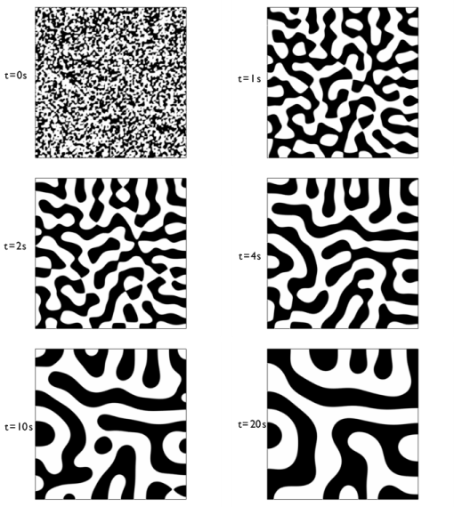
In the Model Builder window, expand the Volume Fraction of Fluid 1 (pf) node, then click Volume Fraction of Fluid 1.
2
In the Settings window for Surface, click to expand the Range section.
3
Select the Manual color range check box.
4
In the Minimum text field, type 0.499.
5
In the Maximum text field, type 0.501.
6
Locate the Coloring and Style section. From the Color table list, choose GrayScale.
7
Right-click Volume Fraction of Fluid 1 and choose Show Legends.
Volume Fraction of Fluid 1 (pf)
1
In the Model Builder window, click Volume Fraction of Fluid 1 (pf).
2
In the Settings window for 2D Plot Group, locate the Data section.
3
From the Time (s) list, choose 0.
4
Click the  Zoom Extents button in the Graphics toolbar.
Compare the resulting plot with that in the upper left panel of Figure 1.To create the remaining plots, plot the solution for the time values 1, 2, 4, 10, and 20 s .
Follow the steps below to reproduce the plot in Figure 2.
Surface Average 1
1
In the Results toolbar, click  More Derived Values and choose Average>Surface Average.
2
3
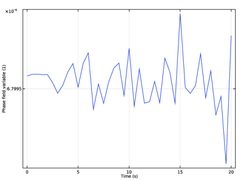
In the Settings window for Surface Average, click Replace Expression in the upper-right corner of the Expressions section. From the menu, choose Component 1 (comp1)>Phase Field>phipf - Phase field variable.
4
Click  Evaluate.
Table
1
Go to the Table window.
2
Click Table Graph in the window toolbar.
Results
Table Graph 1
It can be seen that the mass is conserved throughout the simulation.