PDF

Non-Newtonian Flow
Introduction
This example shows the influence of shear rate dependent viscosity on the flow of a linear polystyrene solution. For this type of flow, you can use the Carreau viscosity model. Due to rotational symmetry, it is possible to reduce the model dimensions from 3D to axisymmetric 2D (see Figure 1).
Model Definition
For Carreau fluid, the constitutive relation between viscous stress K and strain-tensor S is given by
where is the shear rate, μ is the infinite shear rate viscosity, μ0 is the zero shear rate viscosity, λ is a parameter with units of time, and n is a dimensionless parameter.
A solution of linear polystyrene in 1-chloronaphthalene has the properties listed in Table 1 (Ref. 1).
μ
μ0
λ
ρ
The model domain is shown in Figure 1.
Figure 1: Model domain. The geometry can be simplified assuming axisymmetry.
To study the effect on viscosity at different inlet pressures, the model makes use of the parametric solver to vary inlet pressure from 10 kPa to 210 kPa.
Results and Discussion
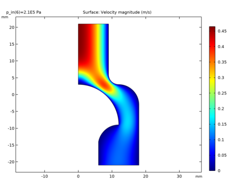
Figure 2 shows that the velocity distribution is more pronounced at the inlet compared to the outlet. This is because the cross section is greater at the outlet. The figure also shows that the region with greatest velocity gradient is in the contraction, which means that the shear rate is largest there.
Figure 2: Velocity field in the modeling domain.
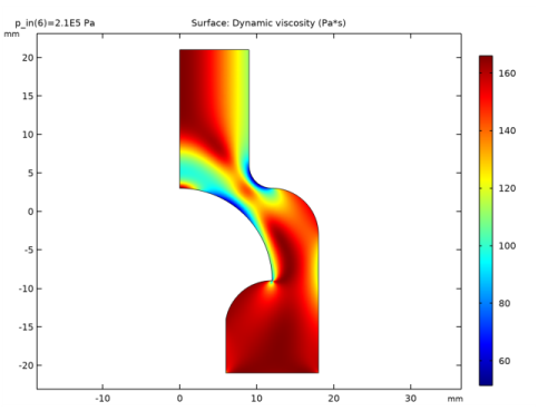
Because the fluid is shear thinning, the viscosity depends on the shear rate and is shown in Figure 3. It reaches its lowest value close to the wall in the contraction between the piston and the wall.
Figure 3: Viscosity distribution in the domain. The lowest viscosity occurs at the wall in the contraction region.
Showing the result of a parametric study of the inlet pressure, Figure 4 contains a cross-sectional plot of the viscosity across the contraction. Sweeping through a range of inlet pressures imposes greater velocities on the non-Newtonian fluid. As the velocity increases, the shear rate also increases and the viscosity decreases. An optimal condition is to have as flat a viscosity profile as possible. This is hindered by also wanting to put through as high a flow rate as possible.
Figure 4: Parametric study of the process, sweeping the inlet pressure from 10 kPa to 210 kPa, while investigating a cross-sectional viscosity plot. A greater inlet pressure (and pressure differential) results in lower values for the viscosity and greater variations in its distribution through the cross section.
Reference
1. R.B. Bird, W.E. Stewart, and E.N. Lightfoot, Transport Phenomena, John Wiley & Sons, 1960.
Application Library path: CFD_Module/Single-Phase_Flow/non_newtonian_flow
Modeling Instructions
From the File menu, choose New.
New
In the New window, click  Model Wizard.
Model Wizard
1
In the Model Wizard window, click  2D Axisymmetric.
2
In the Select Physics tree, select Fluid Flow>Single-Phase Flow>Laminar Flow (spf).
3
Click Add.
4
Click  Study.
5
In the Select Study tree, select General Studies>Stationary.
6
Geometry 1
1
In the Model Builder window, under Component 1 (comp1) click Geometry 1.
2
In the Settings window for Geometry, locate the Units section.
3
From the Length unit list, choose mm.
Polygon 1 (pol1)
1
In the Geometry toolbar, click  Polygon.
2
In the Settings window for Polygon, locate the Object Type section.
3
From the Type list, choose Open curve.
4
Locate the Coordinates section. From the Data source list, choose Vectors.
5
In the r text field, type 0 0 9 9.
6
In the z text field, type 3 21 21 6.
Circular Arc 1 (ca1)
1
In the Geometry toolbar, click  More Primitives and choose Circular Arc.
2
In the Settings window for Circular Arc, locate the Properties section.
3
From the Specify list, choose Endpoints and start angle.
4
Locate the Starting Point section. In the r text field, type 9.
5
In the z text field, type 6.
6
Locate the Endpoint section. In the r text field, type 12.
7
In the z text field, type 3.
8
Locate the Angles section. In the Start angle text field, type 180.
Circular Arc 2 (ca2)
1
In the Geometry toolbar, click  More Primitives and choose Circular Arc.
2
In the Settings window for Circular Arc, locate the Properties section.
3
From the Specify list, choose Endpoints and start angle.
4
Locate the Starting Point section. In the r text field, type 18.
5
In the z text field, type -3.
6
Locate the Endpoint section. In the r text field, type 12.
7
In the z text field, type 3.
Polygon 2 (pol2)
1
In the Geometry toolbar, click  Polygon.
2
In the Settings window for Polygon, locate the Object Type section.
3
From the Type list, choose Open curve.
4
Locate the Coordinates section. From the Data source list, choose Vectors.
5
In the r text field, type 18 18 6 6.
6
In the z text field, type -3 -21 -21 -14.
Circular Arc 3 (ca3)
1
In the Geometry toolbar, click  More Primitives and choose Circular Arc.
2
In the Settings window for Circular Arc, locate the Properties section.
3
From the Specify list, choose Endpoints and start angle.
4
Locate the Starting Point section. In the r text field, type 12.
5
In the z text field, type -9.
6
Locate the Endpoint section. In the r text field, type 6.
7
In the z text field, type -14.
8
Locate the Angles section. In the Start angle text field, type 90.
Circular Arc 4 (ca4)
1
In the Geometry toolbar, click  More Primitives and choose Circular Arc.
2
In the Settings window for Circular Arc, locate the Properties section.
3
From the Specify list, choose Endpoints and start angle.
4
Locate the Starting Point section. In the r text field, type 12.
5
In the z text field, type -9.
6
Locate the Endpoint section. In the z text field, type 3.
Convert to Solid 1 (csol1)
1
In the Geometry toolbar, click  Conversions and choose Convert to Solid.
2
Click in the Graphics window and then press Ctrl+A to select all objects.
3
In the Settings window for Convert to Solid, click  Build All Objects.
4
Click  Build Selected.
5
Click the  Zoom Extents button in the Graphics toolbar.
Form Union (fin)
1
In the Model Builder window, click Form Union (fin).
2
In the Settings window for Form Union/Assembly, click  Build Selected.
Global Definitions
Add a global parameter for the inlet pressure. You will use this as the parameter in a parametric sweep.
Parameters 1
1
In the Model Builder window, under Global Definitions click Parameters 1.
2
In the Settings window for Parameters, locate the Parameters section.
3
Laminar Flow (spf)
Fluid Properties 1
1
In the Model Builder window, under Component 1 (comp1)>Laminar Flow (spf) click Fluid Properties 1.
2
In the Settings window for Fluid Properties, locate the Fluid Properties section.
3
From the ρ list, choose User defined. In the associated text field, type 450.
4
Find the Constitutive relation subsection. From the list, choose Inelastic non-Newtonian.
5
From the Inelastic model list, choose Carreau.
6
From the μ0 list, choose User defined. In the associated text field, type 166.
7
From the μinf list, choose User defined. From the λ list, choose User defined. In the associated text field, type 1.73e-2.
8
From the n list, choose User defined. In the associated text field, type 0.538.
Inlet 1
1
In the Physics toolbar, click  Boundaries and choose Inlet.
2
3
In the Settings window for Inlet, locate the Boundary Condition section.
4
5
Locate the Pressure Conditions section. In the p0 text field, type p_in.
Outlet 1
1
In the Physics toolbar, click  Boundaries and choose Outlet.
2
Mesh 1
1
In the Model Builder window, under Component 1 (comp1) click Mesh 1.
2
In the Settings window for Mesh, locate the Physics-Controlled Mesh section.
3
From the Element size list, choose Extra fine.
4
Click  Build All.
Study 1
Parametric Sweep
1
In the Study toolbar, click  Parametric Sweep.
2
In the Settings window for Parametric Sweep, locate the Study Settings section.
3
4
5
In the Study toolbar, click  Compute.
Results
The default plot groups shows the velocity magnitude in 2D (compare with Figure 2) and 3D as well as the pressure field in 2D.
Visualize the viscosity distribution in a separate plot group with the following steps:
2D Plot Group 4
In the Home toolbar, click  Add Plot Group and choose 2D Plot Group.
Surface 1
1
Right-click 2D Plot Group 4 and choose Surface.
2
In the 2D Plot Group 4 toolbar, click  Plot.
3
Click the  Zoom Extents button in the Graphics toolbar.
4
In the Model Builder window, click Surface 1.
5
In the Settings window for Surface, click Replace Expression in the upper-right corner of the Expression section. From the menu, choose Component 1 (comp1)>Laminar Flow>Material properties>spf.mu_app - Apparent viscosity - Pa·s.
6
In the 2D Plot Group 4 toolbar, click  Plot.
Compare the resulting plot with that in Figure 3.
Apparent Viscosity
1
In the Model Builder window, right-click 2D Plot Group 4 and choose Rename.
2
In the Rename 2D Plot Group dialog box, type Apparent Viscosity in the New label text field.
3
Finally, plot the viscosity across the contraction as in Figure 4.
Cut Line 2D 1
1
In the Results toolbar, click  Cut Line 2D.
2
In the Settings window for Cut Line 2D, locate the Line Data section.
3
In row Point 1, set r to 7.55 and z to 0.32.
4
In row Point 2, set r to 9.97 and z to 3.79.
5
1D Plot Group 5
In the Results toolbar, click  1D Plot Group.
Line Graph 1
1
Right-click 1D Plot Group 5 and choose Line Graph.
2
In the Settings window for Line Graph, locate the Data section.
3
From the Dataset list, choose Cut Line 2D 1.
4
Click Replace Expression in the upper-right corner of the y-Axis Data section. From the menu, choose Component 1 (comp1)>Laminar Flow>Material properties>spf.mu_app - Apparent viscosity - Pa·s.
5
Click to expand the Quality section. From the Recover list, choose Within domains.
6
In the 1D Plot Group 5 toolbar, click  Plot.