Flow Through a Uniform Inclined Screen

PDF

Flow Through a Uniform Inclined Screen

This example simulates the flow through a uniform inclined screen using the Screen feature in Single-Phase Flow physics and compares the results with an analytic solution due to Elder (Ref. 1). The Screen feature is a tool for modeling wire gauzes, perforated plates etc without resolving their geometric complexity (see the CFD Module User’s Guide for further details).

Model Definition

The model geometry is shown in Figure 1.

Figure 1: Model geometry showing flow direction and screen inclination.

Air at a temperature of T = 20 °C enters the channel on the left with a uniform inlet velocity of uin = 1 m/s and exits on the right at uniform pressure, p0 = 0 Pa. The flow through the channel is obstructed by a screen inclined at an angle θ. The combined effect of resistance and refraction (suppression of the tangential velocity component) creates a non-uniform velocity profile on the downstream side of the screen. An asymptotic solution valid for small inclinations is (Ref. 1),

(1)

where K and η are the screen resistance and refraction coefficients. To facilitate comparison with the asymptotic solution, assume that the flow is incompressible and apply free-slip boundary conditions on the channel walls. Choose the user-defined option for both the screen type and refraction in order to set the resistance coefficient K to 2.2 and the refraction coefficient η to 0.78.

Results and Discussion

The study performs a Parametric Sweep with the angle θ taking the values,

Figure 2 shows the outlet velocity scaled according to the left-hand side of Equation 1 together with the asymptotic solution on the right-hand side.

Figure 2: Comparison between the asymptotic solution (blue) and the simulations (red).

The agreement between the asymptotic solution and the simulations is good, surprisingly so even for θ = π/4 (45 °). Figure 3 shows a surface plot of the pressure field together with velocity vectors on the upstream and downstream side of the screen. The velocity vectors are displaced from the screen for clarity. You can easily distinguish the induced pressure jump, the flow distribution and deflection. See Ref. 1 for asymptotic solutions to other related screen-flow problems if you are looking to extend the analysis to screens of varying shape and/or resistance.

Figure 3: Pressure drop, flow distribution and deflection for a screen inclined at an angle of 45 ° to the incoming flow.

Notes About the COMSOL Implementation

The model uses the Screen feature together with a Parametric Sweep to vary the inclination angle of the screen.

1. J.W. Elder, “Steady Flow Through Non-Uniform Gauzes of Arbitrary Shape,” J. Fluid Mech., vol 5, pp 355–363, 1959.

CFD_Module/Verification_Examples/inclined_screen

Modeling Instructions

From the menu, choose .

In the window, click

.

1

In the window, click

.

2

In the tree, select .

3

4

5

In the tree, select .

6

Global Definitions

1

In the window, under click .

2

In the window for , locate the section.

3

In the table, enter the following settings:


Name	Expression	Value	Description
theta	pi/18	0.17453	Angle of inclination
u_in	1[m/s]	1 m/s	Inlet velocity

Rectangle 1 (r1)

1

In the toolbar, click

.

2

In the window for , locate the section.

3

In the text field, type 4.

4

Locate the section. In the text field, type -2.

Polygon 1 (pol1)

1

In the toolbar, click

.

2

In the window for , locate the section.

3

From the list, choose .

4

In the text field, type -0.5*tan(theta) 0.5*tan(theta).

5

In the text field, type 0 1 .

6

In the toolbar, click

.

1

In the toolbar, click

to open the window.

2

Go to the window.

3

In the tree, select .

4

Click in the window toolbar.

5

In the toolbar, click

to close the window.

Laminar Flow (spf)

1

In the window, under click .

2

In the window for , locate the section.

3

From the list, choose .

1

In the toolbar, click

and choose .

2

Select Boundary 1 only.

3

In the window for , locate the section.

4

In the U0 text field, type u_in.

1

In the toolbar, click

and choose .

2

Select Boundary 7 only.

3

In the window for , locate the section.

4

Select the check box.

1

In the toolbar, click

and choose .

2

Select Boundary 4 only.

3

In the window for , locate the section.

4

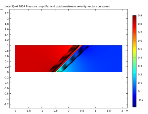
From the list, choose . Locate the section. In the K text field, type 2.2.

5

From the list, choose . In the η text field, type 0.78.

Parametric Sweep

1

In the toolbar, click

.

2

In the window for , locate the section.

3

4

In the table, enter the following settings:


Parameter name	Parameter value list	Parameter unit
theta (Angle of inclination)	pi/18, pi/9, pi/6, 2*pi/9, pi/4

5

In the toolbar, click

.

Create a new plot group to reproduce Figure 2.

1D Plot Group 3

In the toolbar, click

and choose .

1

Right-click and choose .

2

Select Boundary 7 only.

Type in the analytic solution.

3

In the window for , locate the section.

4

In the text field, type 2/pi*log(cot(pi*y/2)).

5

Locate the section. From the list, choose .

6

In the text field, type y.

7

In the toolbar, click

.

1D Plot Group 3

1

In the window, click .

2

In the window for , locate the section.

3

Select the check box.

4

In the text field, type 0.

5

In the text field, type 1.

6

In the text field, type -3.

7

In the text field, type 3.

1

In the window, under right-click and choose .

2

In the window for , locate the section.

3

From the list, choose .

4

From the list, choose .

5

In the list, select .

Scale the solutions for comparison with the analytic solution.

6

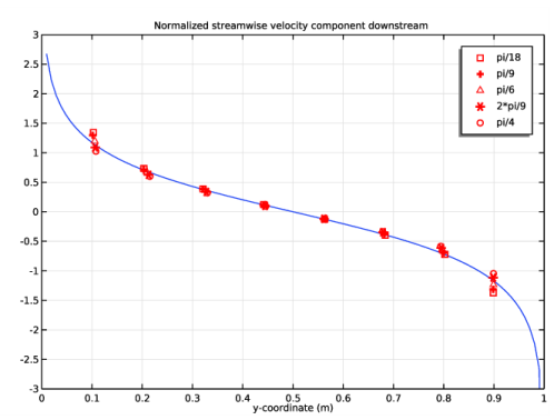
Locate the section. In the text field, type (u/u_in-1)/(1-0.78)/2.2/cos(theta)^2*(1+0.78+2.2*cos(theta)^2)/tan(theta).

7

Click to expand the section. Find the subsection. From the list, choose .

8

From the list, choose .

9

Find the subsection. From the list, choose .

10

Click to expand the section. Select the check box.

11

From the list, choose .

12

In the table, enter the following settings:


Legends
pi/18

1

Right-click and choose .

2

In the window for , locate the section.

3

In the list, select .

4

Locate the section. Find the subsection. From the list, choose .

5

Locate the section. In the table, enter the following settings:


Legends
pi/9

1

Right-click and choose .

2

In the window for , locate the section.

3

In the list, select .

4

Locate the section. Find the subsection. From the list, choose .

5

Locate the section. In the table, enter the following settings:


Legends
pi/6

1

Right-click and choose .

2

In the window for , locate the section.

3

In the list, select .

4

Locate the section. Find the subsection. From the list, choose .

5

Locate the section. In the table, enter the following settings:


Legends
2*pi/9

1

Right-click and choose .

2

In the window for , locate the section.

3

In the list, select .

4

Locate the section. Find the subsection. From the list, choose .

5

Locate the section. In the table, enter the following settings:


Legends
pi/4

1D Plot Group 3

1

In the window, click .

2

In the window for , click to expand the section.

3

From the list, choose .

4

In the toolbar, click

.

5

In the text area, type Normalized streamwise velocity component downstream.

To generate Figure 3, continue with the steps below.

1

In the window, expand the node, then click .

2

In the window for , locate the section.

3

In the text field, type p.

1

In the window, right-click and choose .

2

In the window for , locate the section.

3

In the text field, type up(u).

4

In the text field, type up(v).

5

Locate the section. From the list, choose .

6

Select the check box.

7

In the associated text field, type 0.25.

8

Locate the section. In the text field, type 30.

9

Locate the section. From the list, choose .

1

Right-click and choose .

2

Select Boundary 4 only.

1

In the window, right-click and choose .

2

In the window for , locate the section.

3

In the text field, type -0.05.

4

In the text field, type 0.

5

Locate the section. Select the check box.

6

In the associated text field, type 1.

1

Right-click and choose .

2

In the window for , locate the section.

3

In the text field, type down(u).

4

In the text field, type down(v).

5

Locate the section. From the list, choose .

1

In the window, expand the node, then click .

2

In the window for , locate the section.

3

In the text field, type 0.05.

1

In the window, click .

2

In the window for , click to expand the section.

3

From the list, choose .

4

In the text area, type Pressure drop (Pa) and up/downstream velocity vectors on screen.

5

In the toolbar, click

.