Expansion Fan

Some of the main characteristics of supersonic flows are shock waves and expansion fans. Oblique shock waves take place when a supersonic flow is turned into itself (the area is reduced; see Figure 1), decreasing its Mach number. In Figure 1, the streamlines are deflected upward so that the flow behind the shock is uniform and parallel to the surface. The shock is very thin, which leads to very large gradients of velocity and temperature inside the shock. Hence, a shock wave is a dissipative and irreversible process that generates entropy and decreases the total pressure and total density. However, total temperature is conserved and the static temperature, pressure, and density increase. Note that “total values” refer to the values that the properties of the flow would achieve when brought to stagnation, and “static values” refer to the actual values of the properties evaluated at a certain speed. A special case of oblique shocks is a normal shock, which is perpendicular to the flow direction.

An expansion fan is formed when supersonic flow is turned away from itself (the area is increased; see Figure 1). The direction of the flow changes smoothly and continuously across an expansion wave until it is uniform and parallel to the adjacent surface. Hence entropy is conserved and total conditions do not vary across the wave. The Mach number increases and the static temperature, pressure, and density decrease across the expansion wave.

Figure 1: Oblique shock wave (up) and Prandtl-Meyer expansion fan (down).

This application models an expansion fan at a 15° expansion corner. The inlet flow is supersonic with Mach number 2.5. The flow is assumed to be inviscid and the results are compared with inviscid compressible flow theory. For details about this theory and its implementation in the CFD Module, see the documentation for the model 3D Supersonic Flow in a Channel with a Bump.

Model Definition

The problem is governed by the inviscid compressible flow equations which are modeled by The High Mach Number Flow, Laminar interface in the CFD module in COMSOL Multiphysics. The geometry of the model is depicted in Figure 2.

Figure 2: Model geometry.

Because the flow is assumed to be inviscid, a slip boundary condition is applied at the walls. The inlet flow is supersonic and defined by the free-stream total conditions

The flow is assumed to be supersonic at the outlet.

The fluid is air with a specific gas constant of 287 J/(kg·K) and a ratio of specific heats of 1.4. The dynamic viscosity and the thermal conductivity are set to zero.

Analytical Solution

The forward Mach line (Figure 1) is defined by the inlet Mach angle (see Ref. 1)

(1)

The Mach number after the expansion fan can be obtained from the relation

where ν(M) is the Prandtl-Meyer function

Once M2 is known, the rearward Mach angle is obtained as

The expansion fan is an isentropic process, which produces a continuous and smooth change in the flow. Hence, the total properties are conserved.

Results and Discussion

The distributions of pressure, temperature, and Mach number are depicted in Figure 3 through Figure 5. The flow past the corner is expanded in a succession of infinitesimal waves (Mach waves), decreasing the static pressure and temperature while increasing the Mach number. The streamlines smoothly change their direction across the expansion fan until they are parallel to the surface below.

The Mach number and total properties after the fan are listed in Table 1. The Mach number obtained agrees well with inviscid flow theory, and the total properties of the flow are conserved.

Table 1: Comparison of results.
	Model	Compressible Flow theory
Mach number	3.234	3.234
Total temperature	305.4 K	305.5 K
Total pressure	82.4 kPa	82.7 kPa
Total density	0.940 kg·s	0.943 kg·s

Figure 3: Pressure contours and streamlines.

Figure 4: Mach number.

Figure 5: Temperature contours.

Notes About the COMSOL Implementation

In this model, convergence can be improved using simple tricks. First of all, we have rounded the corner to avoid discontinuities and sharp gradients. Moreover, the adaptive mesh refinement feature is used to refine the mesh at the expansion fan where the gradients are large; see Figure 6.

Figure 6: Adapted mesh. The mesh resolves the expansion fan more finely than the rest of the modeling domain.

Reference

1. J. D. Anderson, Jr., Modern Compressible Flow, McGraw-Hill, 2nd Edition, Singapore 1990.

CFD_Module/High_Mach_Number_Flow/expansion_fan

Modeling Instructions

From the menu, choose .

New

In the window, click

Model Wizard

In the window, click

In the tree, select .

Click .

Click

In the tree, select .

Click

Global Definitions

Parameters 1

In the window, under click .

In the window for , locate the section.

In the table, enter the following settings:


Name	Expression	Value	Description
M1	2.5	2.5	Mach number, inlet
pin_tot	12[psi]	82737 Pa	Total pressure, inlet
Tin_tot	550[R]	305.56 K	Total temperature, inlet
Rs	287[J/kg/K]	287 J/(kg·K)	Specific gas constant
gamma	1.4[1]	1.4	Ratio of specific heats
L_in	3[m]	3 m	Length, inlet
L_wave	4.5[m]	4.5 m	Length after the corner
ht	L_in	3 m	Channel height
R_fillet	0.1[m]	0.1 m	Radius, rounded corner
theta	15[deg]	0.2618 rad	Flow-deflection angle
u_in	M1sqrt(gammaRsTin_tot/(1+0.5M1^2*(-1+gamma))+eps)	583.98 m/s	Velocity, inlet

Geometry 1

Polygon 1 (pol1)

In the toolbar, click

In the window for , locate the section.

From the list, choose .

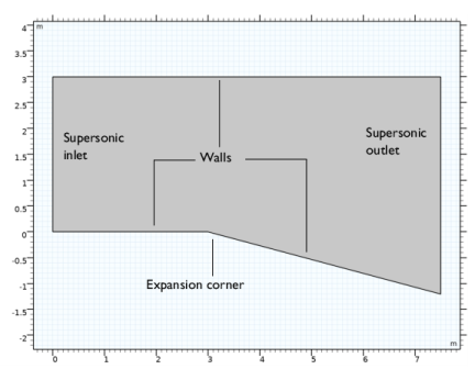
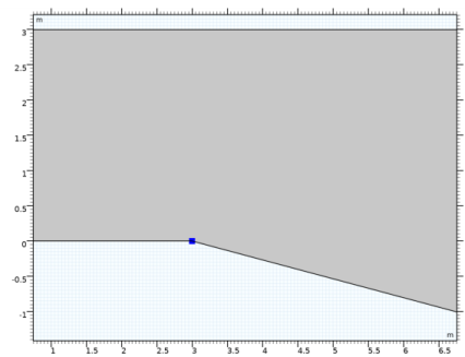
In the text field, type 0, L_in, L_in, L_in+L_wave, L_in+L_wave, L_in+L_wave, L_in+L_wave, 0, 0, 0.

In the text field, type 0, 0, 0, -L_wave*tan(theta), -L_wave*tan(theta), ht, ht, ht, ht, 0.

Fillet 1 (fil1)

In the toolbar, click

On the object , select Point 3 only (expansion corner).

It might be easier to select the correct point by using the window. To open this window, in the toolbar click and choose . (If you are running the cross-platform desktop, you find in the main menu).

In the window for , locate the section.

In the text field, type R_fillet.

Click

Click the

button in the toolbar (see Figure 2)

Definitions

Variables 1

In the window, under right-click and choose .

In the window for , locate the section.

In the table, enter the following settings:


Name	Expression	Unit	Description
v1	sqrt((gamma+1)/(gamma-1))atan(sqrt((gamma-1)(M1^2-1)/(gamma+1)))-atan(sqrt(M1^2-1))	rad	Prandtl-Meyer function, inlet
vi2	sqrt((gamma+1)/(gamma-1))atan(sqrt((gamma-1)(M2^2-1)/(gamma+1)))-atan(sqrt(M2^2-1))		Guess for Prandtl-Meyer function after expansion fan
v2	theta+v1	rad	Residual for global equation
Tin_stat	Tin_tot/(1+0.5M1^2(-1+gamma))	K	Static temperature, inlet
pin_stat	pin_tot/(1+0.5M1^2(-1+gamma))^(gamma/(-1+gamma))	Pa	Static pressure, inlet

The defined variables are used to compute the analytical Mach number and the static conditions at the inlet. M2 will be defined later.

High Mach Number Flow, Laminar (hmnf)

Fluid 1

In the window, under click .

In the window for , locate the section.

From the k list, choose . In the associated text field, type 1e-8.

Locate the section. From the Rs list, choose . In the associated text field, type Rs.

From the γ list, choose .

From the γ list, choose . In the associated text field, type gamma.

Locate the section. From the μ list, choose . In the associated text field, type 1e-8.

The dynamic viscosity and thermal conductivity are set to small values to mimic an inviscid and nonconducting fluid.

Wall 1

In the window, click .

In the window for , locate the section.

From the list, choose .

Slip walls are used for the inviscid case.

Initial Values 1

In the window, click .

In the window for , locate the section.

Specify the u vector as


u_in	x
0	y

In the p text field, type pin_stat.

In the T text field, type Tin_stat.

Inlet 1

In the toolbar, click

and choose .

Select Boundary 1 only (see the supersonic inlet in Figure 2)

In the window for , locate the section.

From the list, choose .

Locate the section. From the list, choose .

In the p0,tot text field, type pin_tot.

In the T0,tot text field, type Tin_tot.

In the Ma0 text field, type M1.

Outlet 1

In the toolbar, click

and choose .

Select Boundary 5 only (see the supersonic outlet in Figure 2)

In the window for , locate the section.

From the list, choose .

Add a global equation to find the analytical Mach number after the expansion fan.

Click the

button in the toolbar.

In the dialog box, in the tree, select the check box for the node .

Click .

Global Equations 1

In the toolbar, click

and choose .

In the window for , locate the section.

In the table, enter the following settings:


Name	f(u,ut,utt,t) (1)	Initial value (u_0) (1)	Initial value (u_t0) (1/s)	Description
M2	v2-vi2	M1	0	Mach flow after the expansion fan, analytical solution

Mesh 1

In the window, under right-click and choose .

Study 1

Step 1: Stationary

In the window, under click .

In the window for , click to expand the section.

From the list, choose .

Solution 1 (sol1)

In the toolbar, click

In the window, expand the node, then click .

In the window for , locate the section.

In the text field, type 1e-5.

Click

Results

Velocity (hmnf)

In the toolbar, click

Streamline 1

In the window, right-click and choose .

Select Boundary 1 only.

In the window for , locate the section.

In the text field, type 10.

Locate the section. Find the subsection. From the list, choose .

From the list, choose .

Select the check box.

In the associated text field, type 1e-3.

From the list, choose .

In the toolbar, click

Click the

button in the toolbar (see Figure 4)

The last step is to compute the Mach number and total values after the expansion fan.

Cut Point 2D 1

In the toolbar, click

In the window for , locate the section.

From the list, choose .

Locate the section. In the text field, type L_in+L_wave.

In the text field, type -L_wave*tan(theta)/2.

Mach number

In the toolbar, click

In the window for , type Mach number in the text field.

Locate the section. From the list, choose .

From the list, choose .

Locate the section. In the table, enter the following settings:


Expression	Unit	Description
hmnf.Ma	1	Mach number

Click

Evaluation points 2-5

Proceed to create evaluation points used to compute the total values of temperature, pressure, and density behind the expansion fan, and the analytical Mach number:


Label	Dataset	Expression
Total pressure	Cut Point 2D 1	p(1+0.5hmnf.Ma^2*(-1+gamma))^(gamma/(-1+gamma))
Total temperature	Cut Point 2D 1	T(1+0.5hmnf.Ma^2*(-1+gamma))
Total density	Cut Point 2D 1	hmnf.rho(1+0.5hmnf.Ma^2*(-1+gamma))^(1/(-1+gamma))
Mach number, analytical solution	Cut Point 2D 1	M2