You are viewing the documentation for an older COMSOL version. The latest version is available here.
PDF

Bimetallic Strip in Airflow
Introduction
This is a conceptual example, illustrating how to couple fluid-structure interaction, heat transfer, and thermal expansion.
A bimetallic strip in an air channel is heated so that it bends. After some time, an airflow with an inlet temperature that varies with time is introduced. As a result, there are changes in deformation caused by both the fluid pressure and the convective cooling. The computed structural deformations are compared for three different cases:
Model Definition
The bimetallic strip geometry consists of two 10 mm x 0.5 cm strips made of copper (lower part) and iron (upper part) materials. The bimetallic strip is placed inside a 70 cm x 10 cm air channel.
Figure 1: Model geometry.
The strip displacements are fixed at the left (upstream) extremity. A 50 W heat source with a uniform distribution is applied to the structure. When the strip is heated, the copper expands more than the iron due to the difference in thermal expansion coefficients. This causes the strip to bend upward.
At the air channel inlet (on the left), the velocity varies with time. Initially there is no flow. After 3000 seconds the inlet velocity is smoothly ramped up to 0.2 m/s.
The inlet temperature is initially set to room temperature (293.15 K). After 5000 seconds it is ramped up to 593.15 K.
Results and Discussion
Figure 2 shows the vertical displacement at the tip of the bimetallic strip as function of time.
Figure 2: Vertical strip tip displacement.
Figure 3 shows the temperature distribution in the channel when there is no imposed airflow.
Figure 3: Velocity (surface) and temperature (contour) in the channel at 3000 s.
Figure 4 shows the temperature distribution in the channel with an airflow cooling the strip. The temperature is significantly decreased and so is the strip tip displacement. The velocity profile in the channel is almost symmetric as the strip has only a small deformation.
 
Figure 4: Velocity (surface) and temperature (contour) in the channel at 5000 s.
Figure 5 shows the temperature distribution and the velocity profile in the channel with hot airflow at the final time step. Now the cooling effect is significantly decreased as the air is warm. The strip deformation clearly changes the flow pattern, and most of the air is passing below the structure.
Figure 5: Velocity (surface) and temperature (contour) in the channel at 7000 s.
Modeling in COMSOL Multiphysics
COMSOL Multiphysics offers the possibility to easily set up this type of combined multiphysics analysis. In the model wizard, you can choose the Fluid-Solid Interaction, Conjugate Heat Transfer multiphysics interface and you will automatically get the multiphysics coupling between the fluid flow, the structural deformation and the heat distribution.
Application Library path: CFD_Module/Fluid-Structure_Interaction/bimetallic_strip_fsi
Modeling Instructions
From the File menu, choose New.
New
In the New window, click  Model Wizard.
Model Wizard
1
In the Model Wizard window, click  2D.
2
In the Select Physics tree, select Fluid Flow>Fluid-Structure Interaction>Conjugate Heat Transfer>Fluid-Solid Interaction.
3
Click Add.
4
Click  Study.
5
In the Select Study tree, select General Studies>Time Dependent.
6
Global Definitions
Parameters 1
1
In the Model Builder window, under Global Definitions click Parameters 1.
2
In the Settings window for Parameters, locate the Parameters section.
3
Geometry 1
Rectangle 1 (r1)
1
In the Geometry toolbar, click  Rectangle.
2
In the Settings window for Rectangle, locate the Size and Shape section.
3
In the Width text field, type ls.
4
In the Height text field, type hs.
5
Locate the Position section. In the y text field, type -hs/2.
6
Click to expand the Layers section. In the table, enter the following settings:
Rectangle 2 (r2)
1
In the Geometry toolbar, click  Rectangle.
2
In the Settings window for Rectangle, locate the Size and Shape section.
3
In the Width text field, type lc.
4
In the Height text field, type hc.
5
Locate the Position section. In the x text field, type -2*ls.
6
In the y text field, type -hc/2.
Form Union (fin)
1
In the Geometry toolbar, click  Build All.
2
Click the  Zoom Extents button in the Graphics toolbar.
Laminar Flow (spf)
1
In the Model Builder window, under Component 1 (comp1) click Laminar Flow (spf).
2
Solid Mechanics (solid)
1
In the Model Builder window, under Component 1 (comp1) click Solid Mechanics (solid).
2
Heat Transfer in Solids and Fluids (ht)
Fluid 1
1
In the Model Builder window, under Component 1 (comp1)>Heat Transfer in Solids and Fluids (ht) click Fluid 1.
2
Definitions
Deforming Domain 1
1
In the Model Builder window, under Component 1 (comp1)>Definitions>Moving Mesh click Deforming Domain 1.
2
Add Material
1
In the Home toolbar, click  Add Material to open the Add Material window.
2
Go to the Add Material window.
3
4
Click  Add to Component 1 (comp1).
5
In the tree, select Built-in>Copper.
6
Click  Add to Component 1 (comp1).
7
In the tree, select Built-in>Iron.
8
Click  Add to Component 1 (comp1).
9
In the Home toolbar, click  Add Material to close the Add Material window.
Materials
Copper (mat2)
1
In the Settings window for Material, locate the Geometric Entity Selection section.
2
Click  Paste Selection.
3
In the Paste Selection dialog box, type 2 in the Selection text field.
4
Iron (mat3)
1
In the Model Builder window, click Iron (mat3).
2
In the Settings window for Material, locate the Geometric Entity Selection section.
3
Click  Paste Selection.
4
In the Paste Selection dialog box, type 3 in the Selection text field.
5
Definitions
Step 1 (step1)
1
In the Home toolbar, click  Functions and choose Local>Step.
2
In the Settings window for Step, type Vinlet in the Function name text field.
3
Locate the Parameters section. In the Location text field, type 3050.
4
In the To text field, type 0.2.
5
Click to expand the Smoothing section. In the Size of transition zone text field, type 100.
Laminar Flow (spf)
In the Model Builder window, under Component 1 (comp1) click Laminar Flow (spf).
Inlet 1
1
In the Physics toolbar, click  Boundaries and choose Inlet.
2
In the Settings window for Inlet, locate the Boundary Condition section.
3
From the list, choose Fully developed flow.
4
Locate the Fully Developed Flow section. In the Uav text field, type Vinlet(t).
5
Outlet 1
1
In the Physics toolbar, click  Boundaries and choose Outlet.
2
Solid Mechanics (solid)
In the Model Builder window, under Component 1 (comp1) click Solid Mechanics (solid).
Fixed Constraint 1
1
In the Physics toolbar, click  Boundaries and choose Fixed Constraint.
2
In the Settings window for Fixed Constraint, locate the Boundary Selection section.
3
Click  Paste Selection.
4
In the Paste Selection dialog box, type 4 6 in the Selection text field.
5
Definitions
Step 2 (step2)
1
In the Home toolbar, click  Functions and choose Local>Step.
2
In the Settings window for Step, type Tinlet in the Function name text field.
3
Locate the Parameters section. In the Location text field, type 5050.
4
In the From text field, type 293.15.
5
In the To text field, type 593.15.
6
Locate the Smoothing section. In the Size of transition zone text field, type 100.
Heat Transfer in Solids and Fluids (ht)
In the Model Builder window, under Component 1 (comp1) click Heat Transfer in Solids and Fluids (ht).
Inflow 1
1
In the Physics toolbar, click  Boundaries and choose Inflow.
2
3
In the Settings window for Inflow, locate the Upstream Properties section.
4
In the Tustr text field, type Tinlet(t).
Outflow 1
1
In the Physics toolbar, click  Boundaries and choose Outflow.
2
Heat Source 1
1
In the Physics toolbar, click  Domains and choose Heat Source.
2
In the Settings window for Heat Source, locate the Domain Selection section.
3
Click  Paste Selection.
4
In the Paste Selection dialog box, type 2 3 in the Selection text field.
5
6
In the Settings window for Heat Source, locate the Heat Source section.
7
In the Q0 text field, type 50[W]/(ls*hs*ht.dz).
Multiphysics
Thermal Expansion 1 (te1)
1
In the Model Builder window, under Component 1 (comp1)>Multiphysics click Thermal Expansion 1 (te1).
2
In the Settings window for Thermal Expansion, locate the Domain Selection section.
3
Click  Paste Selection.
4
In the Paste Selection dialog box, type 2 3 in the Selection text field.
5
Mesh 1
1
In the Model Builder window, under Component 1 (comp1) right-click Mesh 1 and choose Build All.
2
In the Settings window for Mesh, locate the Mesh Settings section.
3
From the Sequence type list, choose User-controlled mesh.
Corner Refinement 1
In the Model Builder window, under Component 1 (comp1)>Mesh 1 right-click Corner Refinement 1 and choose Build Selected.
Mapped 1
1
In the Mesh toolbar, click  Mapped.
2
In the Settings window for Mapped, locate the Domain Selection section.
3
From the Geometric entity level list, choose Domain.
4
Distribution 1
1
Right-click Mapped 1 and choose Distribution.
2
Click the  Zoom Box button in the Graphics toolbar.
3
4
In the Settings window for Distribution, locate the Distribution section.
5
In the Number of elements text field, type 2.
Distribution 2
1
In the Model Builder window, right-click Mapped 1 and choose Distribution.
2
3
In the Settings window for Distribution, locate the Distribution section.
4
In the Number of elements text field, type 100.
5
Click  Build All.
Study 1
Step 1: Time Dependent
1
In the Model Builder window, under Study 1 click Step 1: Time Dependent.
2
In the Settings window for Time Dependent, locate the Study Settings section.
3
In the Output times text field, type range(0,1e2,7e3).
Solution 1 (sol1)
1
In the Study toolbar, click  Show Default Solver.
2
In the Model Builder window, expand the Solution 1 (sol1) node.
3
In the Model Builder window, expand the Study 1>Solver Configurations>Solution 1 (sol1)>Dependent Variables 1 node, then click Pressure (comp1.p).
4
In the Settings window for Field, locate the Scaling section.
5
From the Method list, choose Manual.
6
In the Scale text field, type 0.1.
7
In the Model Builder window, click Spatial mesh displacement (comp1.spatial.disp).
8
In the Settings window for Field, locate the Scaling section.
9
In the Scale text field, type 1e-2.
10
In the Model Builder window, click Temperature (comp1.T).
11
In the Settings window for Field, locate the Scaling section.
12
From the Method list, choose Manual.
13
In the Scale text field, type 600.
14
In the Model Builder window, click Velocity field (spatial frame) (comp1.u_fluid).
15
In the Settings window for Field, locate the Scaling section.
16
From the Method list, choose Manual.
17
In the Scale text field, type 0.5.
18
In the Model Builder window, click Displacement field (comp1.u_solid).
19
In the Settings window for Field, locate the Scaling section.
20
In the Scale text field, type 1e-2.
21
In the Model Builder window, click Time-Dependent Solver 1.
22
In the Settings window for Time-Dependent Solver, click to expand the Time Stepping section.
23
From the Steps taken by solver list, choose Intermediate.
24
In the Model Builder window, expand the Study 1>Solver Configurations>Solution 1 (sol1)>Time-Dependent Solver 1 node, then click Direct.
25
In the Settings window for Direct, locate the General section.
26
From the Solver list, choose PARDISO.
27
In the Model Builder window, expand the Study 1>Solver Configurations>Solution 1 (sol1)>Time-Dependent Solver 1>Segregated 1 node, then click Displacement field.
28
In the Settings window for Segregated Step, click to expand the Method and Termination section.
29
From the Jacobian update list, choose On every iteration.
30
In the Study toolbar, click  Compute.
Results
Velocity (spf)
1
In the Settings window for 2D Plot Group, locate the Color Legend section.
2
From the Position list, choose Bottom.
3
Click the  Zoom Extents button in the Graphics toolbar.
Surface
1
In the Model Builder window, expand the Velocity (spf) node, then click Surface.
2
In the Settings window for Surface, locate the Coloring and Style section.
3
From the Color table list, choose AuroraAustralis.
Contour 1
1
In the Model Builder window, right-click Velocity (spf) and choose Contour.
2
In the Settings window for Contour, locate the Expression section.
3
In the Expression text field, type T.
4
Locate the Coloring and Style section. From the Color table list, choose Thermal.
5
In the Velocity (spf) toolbar, click  Plot.
Pressure (spf)
1
In the Model Builder window, click Pressure (spf).
2
In the Settings window for 2D Plot Group, locate the Color Legend section.
3
From the Position list, choose Bottom.
4
Click the  Zoom Extents button in the Graphics toolbar.
Stress (solid)
1
In the Model Builder window, click Stress (solid).
2
In the Settings window for 2D Plot Group, locate the Color Legend section.
3
From the Position list, choose Bottom.
4
Click the  Zoom Extents button in the Graphics toolbar.
Temperature (ht)
1
In the Model Builder window, click Temperature (ht).
2
In the Settings window for 2D Plot Group, locate the Plot Settings section.
3
From the Frame list, choose Spatial  (x, y, z).
4
Locate the Color Legend section. From the Position list, choose Bottom.
5
Click the  Zoom Extents button in the Graphics toolbar.
Streamline 1
1
Right-click Temperature (ht) and choose Streamline.
2
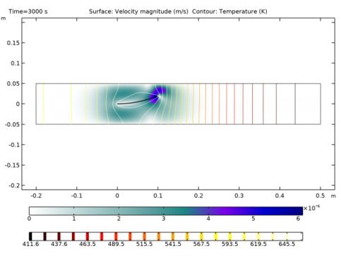
In the Settings window for Streamline, click Replace Expression in the upper-right corner of the Expression section. From the menu, choose Component 1 (comp1)>Laminar Flow>Velocity and pressure>u_fluid,v_fluid - Velocity field (spatial frame).
3
Locate the Streamline Positioning section. From the Positioning list, choose Magnitude controlled.
4
In the Temperature (ht) toolbar, click  Plot.
Isothermal Contours (ht)
1
In the Model Builder window, click Isothermal Contours (ht).
2
In the Settings window for 2D Plot Group, locate the Plot Settings section.
3
From the Frame list, choose Spatial  (x, y, z).
4
Locate the Color Legend section. From the Position list, choose Bottom.
5
Click the  Zoom Extents button in the Graphics toolbar.
Vertical Strip Displacement
1
In the Home toolbar, click  Add Plot Group and choose 1D Plot Group.
2
In the Settings window for 1D Plot Group, type Vertical Strip Displacement in the Label text field.
Point Graph 1
1
Right-click Vertical Strip Displacement and choose Point Graph.
2
In the Settings window for Point Graph, locate the Selection section.
3
Click  Paste Selection.
4
In the Paste Selection dialog box, type 7 in the Selection text field.
5
6
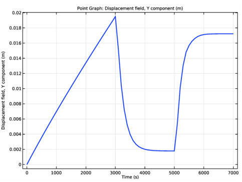
In the Settings window for Point Graph, click Replace Expression in the upper-right corner of the y-Axis Data section. From the menu, choose Component 1 (comp1)>Solid Mechanics>Displacement>Displacement field - m>v_solid - Displacement field, Y component.
7
Click to expand the Coloring and Style section. In the Width text field, type 2.
8
In the Vertical Strip Displacement toolbar, click  Plot.