PDF

Airflow over an Ahmed Body
Introduction
This example describes how to calculate the turbulent flow field around a simple car-like geometry using the CFD Module’s Turbulent Flow, k-ε interface. Detailed instructions guide you through the different steps of the modeling process in COMSOL Multiphysics.
Model Definition
The Ahmed body represents a simplified, ground vehicle geometry of a bluff body type. Its shape is simple enough to allow for accurate flow simulation but retains some important practical features relevant to automobile bodies. The geometry was first defined by Ahmed, who also measured its aerodynamic properties in wind-tunnel experiments (Ref. 1). Further experiments have also been performed by Lienhart and Becker (Ref. 2). The Ahmed body has become a popular benchmark case for RANS models (Ref. 3).
Geometry
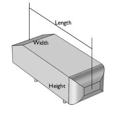
The Ahmed body is presented in Figure 1. The total length (L) of the body is 1.044 m from front to end. It is 0.288 m in height and 0.389 m in width. Cylindrical legs of 0.05 m in length are attached to the bottom surface. The angle of the rear slanting surface is typically varied between 0 and 40 degrees. This particular geometry has a slant angle of 25 degrees, which is the same slant angle used in Ref. 3.
Figure 1: Ahmed body with 25 degree slant of the rear face.
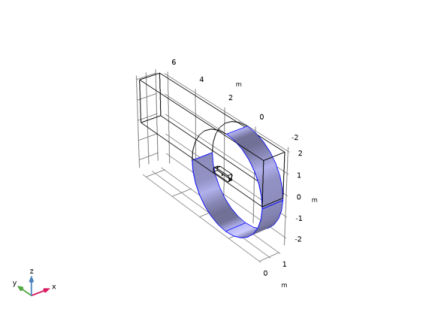
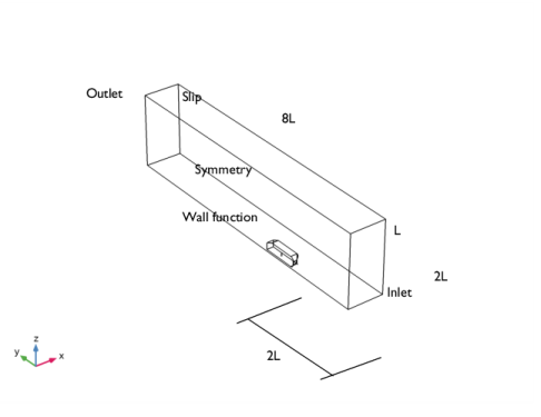
The body is placed in a flow domain that is 8L-by-2L-by-2L (length-by-width-by-height), with its front positioned 2L from the flow inlet face. Mirror symmetry reduces the computational domain by half, as shown in Figure 2.
Figure 2: The size of the computational domain is reduced by mirror symmetry.
Turbulence Model
The Reynolds number based on the length of the body, L, and the inlet velocity is 2.77·106, which means that the flow is turbulent. The k-ε turbulence model is applied to account for the turbulence. The k-ε turbulence model is described in the theory section for the Turbulent Flow interfaces in the CFD Module User’s Guide.
Boundary Conditions
Air enters the computational domain at a freestream velocity u = 40 m/s normal to the inlet surface. Experimental inlet conditions from Ref. 3 are used for the velocity and turbulent kinetic energy. To obtain a condition for ε, Ref. 3 suggests to set μT = 10μ at the inlet. At the outlet, a Pressure condition is applied.
The floor of the flow domain and surface of the Ahmed body are described by wall functions. Wall functions could also be applied to the outer wall and the ceiling of the wind tunnel. Their main effect on the flow around the body is, however, to keep the flow contained; therefore it suffices to model these as slip walls. The temperature is assumed to be 293 K and the reference pressure is 1 atm.
Meshing
A common mesh size in Ref. 3 is half a million cells for simulations with wall functions. However, those simulations do not include the stilts (the legs that support the body), and the computational domains are smaller. Hence, you can expect to need an even larger mesh in this simulation to resolve the flow. How large is, however, difficult to know in advance.
There are two important aspects of the meshing. The first is to resolve the flow in the wake. To achieve this, additional mesh control entities are introduced in the geometry. These entities are advantageous to normal geometrical entities since they are removed once they have been meshed. A smoothing algorithm then smooths the mesh locally in order to minimize gradients in the mesh size. Also, it is easier to introduce a boundary layer mesh when the control entities are removed.
Results and Discussion
A key figure for the Ahmed body is the total drag coefficient, CD, which is defined as
(1)
where F is the total drag force on the body, Ap is area of the body projected on a plane perpendicular to the flow direction (that is, the xz-plane), ρ is the density (approximately equal to 1.2 kg/m3), and u is the freestream velocity (equal to 40 m/s). Ap can be calculated by taking the integral of the y-component of the surface normal vector of the object. By doing so, we find that Ap is equal to 0.059 m2 for the Ahmed body including the stilts. The contributions to CD are commonly reported as the pressure coefficients on front, slant, and base and the skin friction drag coefficient. These numbers are given in Table 1. .
k-ε
As can be seen, most contributions are in reasonable agreements with experiments. The total drag is well predicted, but the individual contributions deviate from experimental values.
The pressure coefficient on the front is too high and the skin friction too low. Ref. 4 uses two different versions of the k-ε model and two different wall function formulations and all combinations show this behavior. It can probably be attributed to the fact that wall functions are not very good at predicting the transition observed in the experiments to take place on the front and roof of the body.
The low value of the slant pressure drag coefficient can be understood by looking at Figure 3, which shows streamlines in the symmetry plane. Experimental results indicate that the flow along the slant is attached almost everywhere and that there are two small recirculation regions behind the base. The computational results capture this behavior, but the extent of the recirculation zones is somewhat overpredicted. The pressure drag coefficient, especially for the slant, is very sensitive to the exact shape and location of the recirculation regions.
Figure 3: Streamlines in the symmetry plane.
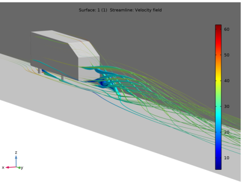
Figure 4 shows a 3D plot of the streamlines behind the Ahmed body. The thickness of the lines is given by the turbulent kinetic energy. The most notable feature of the flow field is an “empty” region behind the body. The streamlines on the edge of the region are thick but with low velocity magnitude. This region is constituted of the recirculation vortices visible in Figure 3. The region ends when vortices from the trailing edges of the body merge into two counterrotating vortices (only one vortex is visible because the other vortex is on the other side of the symmetry plane).
Figure 4: Streamlines behind the Ahmed body. The streamlines are colored by the velocity magnitude and their thickness is proportional to the turbulent kinetic energy.
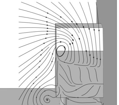
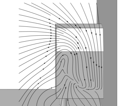
More details are visible in Figure 5 and Figure 6, which show streamlines plots of the velocity in the xz-plane 80 mm and 200 mm downstream of the body, respectively.
Figure 5: Velocity in the xz-plane at y = L + 0.08 m.
The flow pattern 80 mm downstream of the body shows two major vortices, one emanating from the outer edge of the slant and one emanating from the interaction between the floor and the stilts. The flow is qualitatively equal to the experimental results (Ref. 2). There are however quantitative differences. The upper vortex is smaller compared to experiments while the lower vortex is more pronounced than in the experiments.
Figure 6: Velocity in the xz-plane at y = L + 0.20 m.
The flow pattern 200 mm downstream of the body shows that one major vortex is beginning to form but remains of the separate vortices can still be detected. The formation is, however, not proceeded as far as in the experiments.
In conclusion, the major features of the flow are well-captured by the k-ε model, but there are details that deviate from experimental data. This finding is in agreement with other RANS simulations of the Ahmed body (Ref. 3).
References
1. S.R. Ahmed, G. Ramm, and G. Faltin, “Some Salient Features of the Time-Averaged Ground Vehicle Wake,” SAE Technical Paper 840300, 1984.
2. H. Lienhart and S. Becker, “Flow and Turbulence Structure in the Wake of a Simplified Car Model,” SAE 2003 World Congress, SAE Paper 2003-01-0656, Detroit, Michigan, 2003.
3. 9th ERCOFTAC/IAHR Workshop on Refined Turbulence Modelling, Darmstadt University of Technology, Germany, 2001.
4. T.J. Craft, S.E. Gant, H. Iacovides, B.E. Launder, and C.M.E. Robinson, “Computational Study of Flow Around the ‘Ahmed’ Car Body,” 9th ERCOFTAC/IAHR Workshop on Refined Turbulence Modelling, 2001.
Application Library path: CFD_Module/Verification_Examples/ahmed_body
Modeling Instructions
From the File menu, choose New.
New
In the New window, click  Model Wizard.
Model Wizard
1
In the Model Wizard window, click  3D.
2
In the Select Physics tree, select Fluid Flow>Single-Phase Flow>Turbulent Flow>Turbulent Flow, k-ε (spf).
3
Click Add.
4
Click  Study.
5
In the Select Study tree, select General Studies>Stationary.
6
Global Definitions
Parameters 1
1
In the Model Builder window, under Global Definitions click Parameters 1.
2
In the Settings window for Parameters, locate the Parameters section.
3
Geometry 1
Import 1 (imp1)
1
In the Home toolbar, click  Import.
2
In the Settings window for Import, locate the Import section.
3
Click Browse.
4
5
Click Import.
Block 1 (blk1)
1
In the Geometry toolbar, click  Block.
2
In the Settings window for Block, locate the Size and Shape section.
3
In the Width text field, type 2*L.
4
In the Depth text field, type 8*L.
5
In the Height text field, type 2*L.
6
Locate the Position section. In the x text field, type -L.
7
In the y text field, type -2*L.
8
Click  Build Selected.
9
Click the  Go to Default View button in the Graphics toolbar.
10
Click the  Wireframe Rendering button in the Graphics toolbar to view the entire geometry.
Block 2 (blk2)
1
In the Geometry toolbar, click  Block.
2
In the Settings window for Block, locate the Size and Shape section.
3
In the Width text field, type L.
4
In the Depth text field, type 8*L.
5
In the Height text field, type 2*L.
6
Locate the Position section. In the x text field, type -L.
7
In the y text field, type -2*L.
Difference 1 (dif1)
1
In the Geometry toolbar, click  Booleans and Partitions and choose Difference.
2
3
In the Settings window for Difference, locate the Difference section.
4
Find the Objects to subtract subsection. Select the  Activate Selection toggle button.
5
Select the objects blk2 and imp1 only.
All subsequent steps create geometric objects that are only relevant for meshing.
Cylinder 1 (cyl1)
1
In the Geometry toolbar, click  Cylinder.
2
In the Settings window for Cylinder, locate the Object Type section.
3
From the Type list, choose Surface.
4
Locate the Size and Shape section. In the Radius text field, type 2.2*L.
5
In the Height text field, type L.
6
Locate the Position section. In the y text field, type 0.2*L.
7
In the z text field, type -0.1*L.
8
Locate the Axis section. From the Axis type list, choose x-axis.
Delete Entities 1 (del1)
1
In the Model Builder window, right-click Geometry 1 and choose Delete Entities.
2
On the object cyl1, select Boundaries 1, 3, and 4 only.
It might be easier to select the boundaries by using the Selection List window. To open this window, in the Home toolbar click Windows and choose Selection List. (If you are running the cross-platform desktop, you find Windows in the main menu.)
These are all surfaces of the cylinder, except the curved surface behind the body.
Union 1 (uni1)
1
In the Geometry toolbar, click  Booleans and Partitions and choose Union.
2
Click in the Graphics window and then press Ctrl+A to select both objects.
3
In the Settings window for Union, click  Build Selected.
Delete Entities 2 (del2)
1
Right-click Geometry 1 and choose Delete Entities.
2
On the object uni1, select Boundaries 10 and 16 only.
These are the boundaries that protrude above and beneath the channel.
Next, create a domain behind the body. This region will require finer mesh size, because significant turbulence effects are expected.
Work Plane 1 (wp1)
1
In the Geometry toolbar, click  Work Plane.
2
In the Settings window for Work Plane, locate the Plane Definition section.
3
From the Plane type list, choose Face parallel.
4
On the object del2, select Boundary 22 only.
5
Click to expand the Local Coordinate System section. From the Origin list, choose Vertex projection.
6
Find the Vertex for origin subsection. Select the  Activate Selection toggle button.
7
On the object del2, select Point 27 only.
8
In the Rotation text field, type 180.
Work Plane 1 (wp1)>Plane Geometry
In the Model Builder window, click Plane Geometry.
Work Plane 1 (wp1)>Polygon 1 (pol1)
1
In the Work Plane toolbar, click  Polygon.
2
In the Settings window for Polygon, locate the Coordinates section.
3
From the Data source list, choose Vectors.
4
In the xw text field, type 0 Sb Sb H_body H_body H_body H_body 0.
5
In the yw text field, type 0 0 0 -Rl -Rl L L L.
6
In the Work Plane toolbar, click  Build All.
Extrude 1 (ext1)
1
In the Model Builder window, under Component 1 (comp1)>Geometry 1 right-click Work Plane 1 (wp1) and choose Extrude.
2
In the Settings window for Extrude, locate the Distances section.
3
4
Click  Build All Objects.
Ignore Edges 1 (ige1)
1
In the Geometry toolbar, click  Virtual Operations and choose Ignore Edges.
2
On the object fin, select Edges 36, 41, 46, and 47 only, which belong to the cylindrical legs.
Mesh Control Domains 1 (mcd1)
1
In the Geometry toolbar, click  Virtual Operations and choose Mesh Control Domains.
2
On the object ige1, select Domain 2 only.
Mesh Control Faces 1 (mcf1)
1
In the Geometry toolbar, click  Virtual Operations and choose Mesh Control Faces.
2
Click the  Zoom Extents button in the Graphics toolbar.
3
On the object mcd1, select Boundary 12 only.
4
In the Geometry toolbar, click  Build All.
The model geometry is now complete. Compare with Figure 2.
Global Definitions
Create an interpolation function from data available in a file. This function provides data for the turbulent kinetic energy at the inlet.
Interpolation 1 (int1)
1
In the Home toolbar, click  Functions and choose Global>Interpolation.
2
In the Settings window for Interpolation, locate the Definition section.
3
From the Data source list, choose File.
4
Click Browse.
5
6
Click Import.
7
Find the Functions subsection. In the table, enter the following settings:
8
Locate the Units section. In the Arguments text field, type m.
9
In the Function text field, type m^2/s^2.
Create an explicit selection of the boundaries of the body.
Definitions
Body
1
In the Definitions toolbar, click  Explicit.
2
In the Settings window for Explicit, type Body in the Label text field.
3
Locate the Input Entities section. From the Geometric entity level list, choose Boundary.
4
Click the  Select Box button in the Graphics toolbar.
Use the Select box tool to mark all boundaries that belong to the body, which corresponds to:
5
Add Material
1
In the Home toolbar, click  Add Material to open the Add Material window.
2
Go to the Add Material window.
3
4
Click Add to Component in the window toolbar.
5
In the Home toolbar, click  Add Material to close the Add Material window.
Turbulent Flow, k-ε (spf)
Wall 2
1
In the Model Builder window, under Component 1 (comp1) right-click Turbulent Flow, k-ε (spf) and choose Wall.
2
In the Settings window for Wall, locate the Boundary Condition section.
3
From the Wall condition list, choose Slip.
4
Symmetry 1
1
In the Physics toolbar, click  Boundaries and choose Symmetry.
2
Inlet 1
1
In the Physics toolbar, click  Boundaries and choose Inlet.
2
3
In the Settings window for Inlet, locate the Turbulence Conditions section.
4
Click the Specify turbulence variables button.
5
In the k0 text field, type kin(x,z).
6
In the ε0 text field, type spf.C_mu*kin(x,z)^2*spf.rho/(10*1.814e-5[Pa*s]).
7
Locate the Velocity section. Click the Velocity field button.
8
Specify the u0 vector as
Change to unidirectional constraints to avoid reaction forces in the pressure from the constraint for ε.
9
Click the  Show More Options button in the Model Builder toolbar.
10
In the Show More Options dialog box, in the tree, select the check box for the node Physics>Advanced Physics Options.
11
12
In the Settings window for Inlet, click to expand the Constraint Settings section.
13
From the Apply reaction terms on list, choose Individual dependent variables.
Outlet 1
1
In the Physics toolbar, click  Boundaries and choose Outlet.
2
Define variables and integration operators to calculate the drag and pressure coefficients.
Definitions
Integration 1 (intop1)
In the Definitions toolbar, click  Nonlocal Couplings and choose Integration.
Add a nonlocal integration coupling for all surfaces on the Ahmed body.
1
In the Settings window for Integration, type Id in the Operator name text field.
2
Locate the Source Selection section. From the Geometric entity level list, choose Boundary.
3
Click  Paste Selection.
4
In the Paste Selection dialog box, type 5-11, 13-16 in the Selection text field.
5
Add a nonlocal integration coupling for the slant.
Integration 2 (intop2)
1
In the Definitions toolbar, click  Nonlocal Couplings and choose Integration.
2
In the Settings window for Integration, type Is in the Operator name text field.
3
Locate the Source Selection section. From the Geometric entity level list, choose Boundary.
4
Click  Paste Selection.
5
In the Paste Selection dialog box, type 10 in the Selection text field.
6
Add a nonlocal integration coupling for the front.
Integration 3 (intop3)
1
In the Definitions toolbar, click  Nonlocal Couplings and choose Integration.
2
In the Settings window for Integration, type Ik in the Operator name text field.
3
Locate the Source Selection section. From the Geometric entity level list, choose Boundary.
4
Click  Paste Selection.
5
In the Paste Selection dialog box, type 5 6 7 13 in the Selection text field.
6
Add a nonlocal integration coupling for the base.
Integration 4 (intop4)
1
In the Definitions toolbar, click  Nonlocal Couplings and choose Integration.
2
In the Settings window for Integration, type Ib in the Operator name text field.
3
Locate the Source Selection section. From the Geometric entity level list, choose Boundary.
4
Click  Paste Selection.
5
In the Paste Selection dialog box, type 11 in the Selection text field.
6
Variables 1
1
In the Model Builder window, right-click Definitions and choose Variables.
2
In the Settings window for Variables, locate the Variables section.
3
In the expression for the skin friction, the wall function equation is used directly for maximum accuracy.
Mesh 1
Size
1
In the Model Builder window, under Component 1 (comp1) right-click Mesh 1 and choose Edit Physics-Induced Sequence.
2
In the Settings window for Size, locate the Element Size section.
3
Click the Custom button.
4
Locate the Element Size Parameters section. In the Maximum element size text field, type 0.1.
5
In the Minimum element size text field, type 0.0025.
6
In the Curvature factor text field, type 0.4.
7
In the Resolution of narrow regions text field, type 0.25.
Size 1
1
In the Model Builder window, click Size 1.
2
In the Settings window for Size, locate the Geometric Entity Selection section.
3
Click  Clear Selection.
4
5
Locate the Element Size section. Click the Custom button.
6
Locate the Element Size Parameters section. Select the Maximum element size check box.
7
8
Click  Build Selected.
Size 2
1
In the Model Builder window, right-click Mesh 1 and choose Size.
2
In the Settings window for Size, locate the Geometric Entity Selection section.
3
From the Geometric entity level list, choose Boundary.
4
5
Locate the Element Size section. Click the Custom button.
6
Locate the Element Size Parameters section. Select the Maximum element size check box.
7
Size 3
1
Right-click Mesh 1 and choose Size.
2
In the Settings window for Size, locate the Geometric Entity Selection section.
3
From the Geometric entity level list, choose Boundary.
4
5
Locate the Element Size section. Click the Custom button.
6
Locate the Element Size Parameters section. Select the Maximum element size check box.
7
Size 4
1
Right-click Mesh 1 and choose Size.
2
In the Settings window for Size, locate the Geometric Entity Selection section.
3
From the Geometric entity level list, choose Boundary.
4
5
Locate the Element Size section. Click the Custom button.
6
Locate the Element Size Parameters section. Select the Maximum element size check box.
7
Size 5
1
Right-click Mesh 1 and choose Size.
2
In the Settings window for Size, locate the Geometric Entity Selection section.
3
From the Geometric entity level list, choose Edge.
4
5
Locate the Element Size section. Click the Custom button.
6
Locate the Element Size Parameters section. Select the Maximum element size check box.
7
Corner Refinement 1
In the Model Builder window, right-click Corner Refinement 1 and choose Disable.
Free Tetrahedral 1
1
In the Model Builder window, click Free Tetrahedral 1.
2
In the Settings window for Free Tetrahedral, locate the Domain Selection section.
3
From the Geometric entity level list, choose Domain.
4
Size 1
1
Right-click Free Tetrahedral 1 and choose Size.
2
In the Settings window for Size, locate the Element Size section.
3
Click the Custom button.
4
Locate the Element Size Parameters section. Select the Maximum element growth rate check box.
5
Free Tetrahedral 1
Right-click Free Tetrahedral 1 and choose Build Selected.
Free Tetrahedral 2
1
In the Mesh toolbar, click  Free Tetrahedral.
2
In the Settings window for Free Tetrahedral, locate the Domain Selection section.
3
From the Geometric entity level list, choose Domain.
4
5
Click  Build Selected.
Boundary Layers 1
1
In the Model Builder window, click Boundary Layers 1.
2
In the Settings window for Boundary Layers, locate the Geometric Entity Selection section.
3
Click  Clear Selection.
4
Boundary Layer Properties 1
1
In the Model Builder window, expand the Boundary Layers 1 node, then click Boundary Layer Properties 1.
2
In the Settings window for Boundary Layer Properties, locate the Boundary Layer Properties section.
3
In the Number of boundary layers text field, type 6.
4
In the Thickness adjustment factor text field, type 1.5.
Boundary Layers 1
In the Model Builder window, right-click Boundary Layers 1 and choose Build Selected.
Swept 1
1
In the Mesh toolbar, click  Swept.
2
In the Settings window for Swept, locate the Domain Selection section.
3
From the Geometric entity level list, choose Domain.
4
Distribution 1
1
Right-click Swept 1 and choose Distribution.
2
In the Settings window for Distribution, locate the Distribution section.
3
From the Distribution type list, choose Predefined.
4
In the Number of elements text field, type 28.
5
In the Element ratio text field, type 6.
6
In the Model Builder window, right-click Mesh 1 and choose Build All.
Study 1
1
In the Home toolbar, click  Compute.
It is advisable to disable automatic update of plots when working with large 3D models.
Results
1
In the Model Builder window, click Results.
2
In the Settings window for Results, locate the Update of Results section.
3
Select the Only plot when requested check box.
Wall Resolution (spf)
Investigate the lift-off in viscous units to verify that the Wall Resolution is sufficient.
1
In the Model Builder window, under Results click Wall Resolution (spf).
2
In the Settings window for 3D Plot Group, locate the Plot Settings section.
3
From the View list, choose New view.
4
In the Wall Resolution (spf) toolbar, click  Plot.
Use the mouse to zoom and rotate to obtain the image below.
The wall lift-off is reasonably close to the target value of 11.06 on most of the body, and can hence be considered to be acceptable.
Create a new dataset of the boundaries of the body, bottom, and the symmetry plane. It will be used by different plots for better visualization of the result.
Plot surfaces
1
In the Results toolbar, click  More Datasets and choose Surface.
2
In the Settings window for Surface, locate the Selection section.
3
From the Selection list, choose Body and add the bottom and back boundary (boundaries 1 and 3).
4
5
In the Label text field, type Plot surfaces.
Slice
1
In the Model Builder window, expand the Results>Velocity (spf) node, then click Slice.
2
In the Settings window for Slice, locate the Plane Data section.
3
From the Entry method list, choose Coordinates.
4
In the x-coordinates text field, type 0.15.
5
Locate the Coloring and Style section. From the Color table list, choose Disco.
6
Select the Reverse color table check box.
Velocity (spf)
1
In the Model Builder window, click Velocity (spf).
2
In the Settings window for 3D Plot Group, locate the Plot Settings section.
3
Clear the Plot dataset edges check box.
Surface 1
1
Right-click Velocity (spf) and choose Surface.
2
In the Settings window for Surface, locate the Data section.
3
From the Dataset list, choose Plot surfaces.
4
Locate the Expression section. In the Expression text field, type 1.
5
Locate the Coloring and Style section. From the Coloring list, choose Uniform.
6
From the Color list, choose Gray.
7
Click the  Go to YZ View button in the Graphics toolbar and use the mouse to zoom in.
Velocity (spf)
1
In the Model Builder window, click Velocity (spf).
2
In the Settings window for 3D Plot Group, locate the Plot Settings section.
3
From the View list, choose New view.
4
In the Velocity (spf) toolbar, click  Plot.
The slice plot of the velocity clearly shows the recirculation zone behind the body. The result looks smooth which further supports the assumption that the resolution is acceptable.
To calculate the entries in Table 1, perform the following steps:
Global Evaluation 1
1
In the Model Builder window, expand the Results>Derived Values node.
2
Right-click Derived Values and choose Global Evaluation.
3
In the Settings window for Global Evaluation, locate the Expressions section.
4
5
Click  Evaluate.
The following steps reproduce Figure 3:
Symmetry plane
1
In the Results toolbar, click  More Datasets and choose Surface.
2
In the Settings window for Surface, type Symmetry plane in the Label text field.
3
Locate the Parameterization section. From the x- and y-axes list, choose yz-plane.
4
Streamlines 2D
1
In the Results toolbar, click  2D Plot Group.
2
In the Settings window for 2D Plot Group, type Streamlines 2D in the Label text field.
3
Locate the Data section. From the Dataset list, choose Symmetry plane.
Streamline 1
1
Right-click Streamlines 2D and choose Streamline.
2
In the Settings window for Streamline, locate the Expression section.
3
In the x component text field, type v.
4
In the y component text field, type w.
5
Locate the Streamline Positioning section. In the Points text field, type 31.
6
In the Streamlines 2D toolbar, click  Plot.
Streamlines 2D
1
In the Model Builder window, click Streamlines 2D.
2
Streamlines 3D
The following steps reproduce Figure 4:
1
In the Home toolbar, click  Add Plot Group and choose 3D Plot Group.
2
In the Settings window for 3D Plot Group, type Streamlines 3D in the Label text field.
3
Locate the Plot Settings section. Clear the Plot dataset edges check box.
Surface 1
1
Right-click Streamlines 3D and choose Surface.
2
In the Settings window for Surface, locate the Data section.
3
From the Dataset list, choose Plot surfaces.
4
Locate the Expression section. In the Expression text field, type 1.
5
Locate the Coloring and Style section. From the Coloring list, choose Uniform.
6
From the Color list, choose Gray.
Streamline 1
1
In the Model Builder window, right-click Streamlines 3D and choose Streamline.
2
In the Settings window for Streamline, locate the Streamline Positioning section.
3
From the Positioning list, choose Starting-point controlled.
4
From the Entry method list, choose Coordinates.
5
In the x text field, type range(0.01,0.03,0.16) range(0.01,0.03,0.16) range(0.01,0.03,0.16) range(0.01,0.03,0.16) range(0.01,0.03,0.16).
6
In the y text field, type -0.5*L.
7
In the z text field, type 0.02*1^range(1,6) 0.08*1^range(1,6) 0.14*1^range(1,6) 0.2*1^range(1,6) 0.26*1^range(1,6).
8
Locate the Coloring and Style section. Find the Line style subsection. From the Type list, choose Tube.
9
In the Tube radius expression text field, type k*1[s^2/m].
10
Select the Radius scale factor check box.
11
Color Expression 1
Right-click Streamline 1 and choose Color Expression.
Streamlines 3D
1
In the Settings window for 3D Plot Group, locate the Plot Settings section.
2
From the View list, choose New view.
3
In the Streamlines 3D toolbar, click  Plot.
The following steps will reproduce figures Figure 5 and Figure 6:
Cut Plane 80 mm
1
In the Results toolbar, click  Cut Plane.
2
In the Settings window for Cut Plane, type Cut Plane 80†mm in the Label text field.
3
Locate the Plane Data section. From the Plane list, choose zx-planes.
4
In the y-coordinate text field, type L+0.08.
Cut Plane 200 mm
1
In the Results toolbar, click  Cut Plane.
2
In the Settings window for Cut Plane, type Cut Plane 200†mm in the Label text field.
3
Locate the Plane Data section. From the Plane list, choose zx-planes.
4
In the y-coordinate text field, type L+0.2.
Streamline: Velocity in xz-plane, 80 mm
1
In the Results toolbar, click  3D Plot Group.
2
In the Settings window for 3D Plot Group, type Streamline: Velocity in xz-plane, 80†mm in the Label text field.
3
Click to expand the Title section.
Streamline Surface 1
1
In the Streamline: Velocity in xz-plane, 80†mm toolbar, click  More Plots and choose Streamline Surface.
2
In the Settings window for Streamline Surface, locate the Data section.
3
From the Dataset list, choose Cut Plane 80 mm.
4
Locate the Streamline Positioning section. From the Positioning list, choose Uniform density.
5
In the Separating distance text field, type 0.04.
6
Locate the Coloring and Style section. Find the Line style subsection. From the Type list, choose Tube.
7
Select the Radius scale factor check box.
8
9
Find the Point style subsection. From the Type list, choose Arrow.
10
Select the Number of arrows check box.
11
12
From the Arrow length list, choose Logarithmic.
13
In the Range quotient text field, type 1000.
14
Select the Scale factor check box.
15
16
From the Color list, choose Black.
Filter 1
1
Right-click Streamline Surface 1 and choose Filter.
2
In the Settings window for Filter, locate the Element Selection section.
3
In the Logical expression for inclusion text field, type (x<0.35)*(z<0.45).
Surface 1
1
In the Model Builder window, right-click Streamline: Velocity in xz-plane, 80 mm and choose Surface.
2
In the Settings window for Surface, locate the Data section.
3
From the Dataset list, choose Plot surfaces.
4
Locate the Expression section. In the Expression text field, type 1.
5
Locate the Coloring and Style section. From the Coloring list, choose Uniform.
6
From the Color list, choose Gray.
Streamline: Velocity in xz-plane, 80 mm
1
In the Model Builder window, click Streamline: Velocity in xz-plane, 80 mm.
2
In the Settings window for 3D Plot Group, locate the Plot Settings section.
3
From the View list, choose New view.
4
In the Streamline: Velocity in xz-plane, 80†mm toolbar, click  Plot.
Duplicate the last plot and modify the settings to obtain the results at 200 mm.
Streamline: Velocity in xz-plane, 200 mm
1
Right-click Streamline: Velocity in xz-plane, 80 mm and choose Duplicate.
2
In the Model Builder window, click Streamline: Velocity in xz-plane, 80 mm 1.
3
In the Settings window for 3D Plot Group, type Streamline: Velocity in xz-plane, 200†mm in the Label text field.
Streamline Surface 1
1
In the Model Builder window, click Streamline Surface 1.
2
In the Settings window for Streamline Surface, locate the Data section.
3
From the Dataset list, choose Cut Plane 200 mm.
Streamline: Velocity in xz-plane, 200 mm
1
In the Model Builder window, click Streamline: Velocity in xz-plane, 200 mm.
2
In the Streamline: Velocity in xz-plane, 200†mm toolbar, click  Plot.