|
|
|


|
1
|
|
2
|
|
3
|
Click Add.
|
|
4
|
Click
|
|
5
|
|
6
|
Click
|
|
1
|
|
2
|
|
3
|
|
4
|
|
5
|
|
1
|
|
2
|
|
3
|
|
4
|
Browse to the model’s Application Libraries folder and double-click the file pb_flow_battery_parameters.txt.
|
|
1
|
|
2
|
|
3
|
|
1
|
|
2
|
|
3
|
|
1
|
|
2
|
|
3
|
|
1
|
|
2
|
|
3
|
|
1
|
|
2
|
|
3
|
|
4
|
|
5
|
|
1
|
In the Model Builder window, under Component 1 (comp1) right-click Laminar Flow (spf) and choose Inlet.
|
|
2
|
|
3
|
|
4
|
|
5
|
|
1
|
|
2
|
|
3
|
|
4
|
|
1
|
|
1
|
|
2
|
|
3
|
|
4
|
|
5
|
|
1
|
|
1
|
|
2
|
|
3
|
|
1
|
|
3
|
|
4
|
|
5
|
|
6
|
|
7
|
|
1
|
|
2
|
|
3
|
|
4
|
|
5
|
|
1
|
|
2
|
|
1
|
|
2
|
|
3
|
In the tree, select Electrochemistry>Tertiary Current Distribution, Nernst-Planck>Tertiary, Electroneutrality (tcd).
|
|
4
|
|
5
|
In the Concentrations table, enter the following settings:
|
|
6
|
Find the Physics interfaces in study subsection. In the table, clear the Solve check box for Study 1.
|
|
7
|
|
8
|
|
9
|
|
10
|
|
11
|
|
1
|
|
2
|
|
3
|
|
4
|
|
5
|
|
1
|
|
2
|
|
3
|
|
4
|
|
5
|
|
1
|
|
2
|
|
3
|
|
4
|
|
5
|
|
1
|
|
2
|
|
3
|
Locate the Parameters section. In the Lower limit text field, type t_charge+t_rest+t_discharge+t_rest.
|
|
4
|
|
5
|
|
1
|
|
2
|
|
3
|
|
4
|
Browse to the model’s Application Libraries folder and double-click the file pb_flow_battery_variables.txt.
|
|
1
|
In the Model Builder window, under Component 1 (comp1) click Tertiary Current Distribution, Nernst-Planck (tcd).
|
|
2
|
In the Settings window for Tertiary Current Distribution, Nernst-Planck, locate the Electrolyte Charge Conservation section.
|
|
3
|
|
1
|
In the Model Builder window, under Component 1 (comp1)>Tertiary Current Distribution, Nernst-Planck (tcd) click Electrolyte 1.
|
|
2
|
|
3
|
|
4
|
|
5
|
|
6
|
|
7
|
|
8
|
|
9
|
|
1
|
|
2
|
|
3
|
|
4
|
|
5
|
|
6
|
|
1
|
|
2
|
|
3
|
|
1
|
|
2
|
|
3
|
|
1
|
|
2
|
|
3
|
|
4
|
|
5
|
Locate the Electrode Kinetics section. From the Exchange current density type list, choose Lumped multistep.
|
|
6
|
|
γ? (1)
|
|
|
8
|
|
9
|
|
1
|
|
2
|
|
3
|
|
4
|
Locate the Electrode Phase Potential Condition section. From the Electrode phase potential condition list, choose Average current density.
|
|
5
|
|
6
|
|
1
|
|
2
|
|
3
|
|
4
|
|
5
|
|
6
|
|
7
|
|
8
|
Locate the Electrode Kinetics section. From the Exchange current density type list, choose Lumped multistep.
|
|
9
|
|
γ? (1)
|
|
|
1
|
In the Model Builder window, under Component 1 (comp1)>Tertiary Current Distribution, Nernst-Planck (tcd)>Positive Electrode click Electrode Reaction 1.
|
|
2
|
|
1
|
In the Model Builder window, under Component 1 (comp1)>Tertiary Current Distribution, Nernst-Planck (tcd)>Positive Electrode click Electrode Reaction 2.
|
|
2
|
|
3
|
|
4
|
|
5
|
Locate the Equilibrium Potential section. From the Eeq list, choose User defined. Locate the Electrode Kinetics section. From the iloc,expr list, choose User defined. In the associated text field, type i_PbO.
|
|
1
|
|
2
|
In the Settings window for Electrode Surface, click to expand the Dissolving-Depositing Species section.
|
|
3
|
Click
|
|
4
|
Click
|
|
1
|
|
2
|
|
3
|
In the Stoichiometric coefficients for dissolving-depositing species: table, enter the following settings:
|
|
1
|
|
2
|
|
3
|
In the Stoichiometric coefficients for dissolving-depositing species: table, enter the following settings:
|
|
1
|
|
2
|
|
3
|
|
4
|
|
5
|
|
1
|
|
2
|
|
3
|
|
4
|
|
1
|
|
2
|
|
3
|
|
4
|
|
1
|
|
2
|
|
3
|
|
4
|
|
1
|
In the Model Builder window, under Component 1 (comp1)>Global ODEs and DAEs (ge) click Global Equations 1.
|
|
2
|
|
4
|
|
5
|
|
6
|
Click
|
|
7
|
|
8
|
Click OK.
|
|
9
|
|
10
|
|
11
|
|
12
|
Click
|
|
13
|
|
14
|
Click OK.
|
|
1
|
|
2
|
|
3
|
|
4
|
|
1
|
|
2
|
|
3
|
|
4
|
|
1
|
|
2
|
|
3
|
|
4
|
|
1
|
|
2
|
|
3
|
|
4
|
|
1
|
|
2
|
|
3
|
|
4
|
|
1
|
|
2
|
|
3
|
|
4
|
|
1
|
|
2
|
|
3
|
|
4
|
Locate the Physics and Variables Selection section. In the table, clear the Solve for check box for Laminar Flow (spf).
|
|
5
|
Click to expand the Values of Dependent Variables section. Find the Values of variables not solved for subsection. From the Settings list, choose User controlled.
|
|
6
|
|
7
|
|
8
|
|
1
|
|
2
|
|
3
|
In the Model Builder window, expand the Study 2>Solver Configurations>Solution 2 (sol2)>Dependent Variables 1 node, then click Concentration (comp1.cH).
|
|
4
|
|
5
|
|
6
|
|
7
|
|
8
|
|
9
|
|
10
|
|
11
|
|
12
|
|
13
|
|
14
|
|
15
|
|
16
|
|
17
|
|
18
|
|
19
|
|
1
|
|
2
|
|
1
|
|
2
|
|
3
|
|
4
|
|
5
|
|
6
|
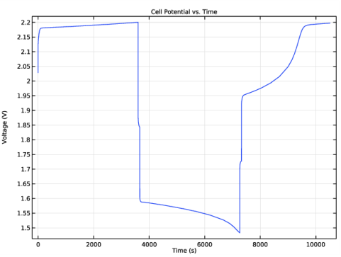
In the associated text field, type Voltage (V).
|
|
1
|
|
2
|
|
3
|
|
4
|
|
1
|
|
2
|
|
3
|
|
4
|
|
1
|
|
2
|
|
3
|
|
4
|
|
5
|
|
6
|
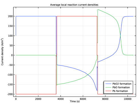
In the associated text field, type Current density (A/m<sup>2</sup>).
|
|
7
|
|
1
|
|
2
|
|
3
|
|
4
|
In the Columns list, choose Local current density (A/m^2), Boundary Probe 2, Local current density (A/m^2), Boundary Probe 3, and Local current density (A/m^2), Boundary Probe 4.
|
|
5
|
|
6
|
|
8
|
|
9
|
|
1
|
|
2
|
|
1
|
|
2
|
|
3
|
|
4
|
|
5
|
|
6
|
In the associated text field, type Time (s).
|
|
7
|
|
8
|
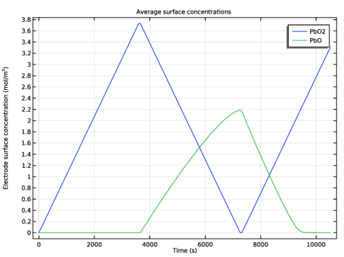
In the associated text field, type Electrode surface concentration (mol/m<sup>2</sup>).
|
|
1
|
|
2
|
|
3
|
|
4
|
In the Columns list, choose Dissolving-depositing species concentration , 1 component (mol/m^2), Boundary Probe 5 and Dissolving-depositing species concentration , 2 component (mol/m^2), Boundary Probe 6.
|
|
5
|
|
6
|
|
8
|
|
9
|
|
1
|
|
2
|
|
1
|
|
2
|
|
3
|
|
4
|
|
5
|
|
6
|
|
7
|
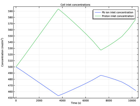
In the associated text field, type Concentration (mol/m<sup>3</sup>).
|
|
1
|
|
2
|
|
3
|
|
4
|
|
1
|
|
2
|
In the Settings window for Surface, click Replace Expression in the upper-right corner of the Expression section. From the menu, choose Component 1 (comp1)>Tertiary Current Distribution, Nernst-Planck>Species cH>cH - Concentration - mol/m³.
|
|
1
|
|
2
|
|
3
|
|
1
|
|
2
|
In the Settings window for 2D Plot Group, type H+ Concentration Distribution in the Label text field.
|
|
3
|
|
4
|
|
5
|
|
1
|
|
2
|
|
3
|
|
1
|
|
2
|
In the Settings window for Surface, click Replace Expression in the upper-right corner of the Expression section. From the menu, choose Component 1 (comp1)>Tertiary Current Distribution, Nernst-Planck>Species cPbII>cPbII - Concentration - mol/m³.
|
|
3
|
|
4
|
|
1
|
|
2
|
In the Settings window for 2D Plot Group, type PbII Concentration Distribution in the Label text field.
|
|
3
|
|
4
|
|
5
|
|
1
|
|
2
|
|
1
|
|
2
|
|
3
|
|
4
|
|
5
|