|
|
|

|
1
|
|
2
|
|
3
|
Click Add.
|
|
4
|
Click
|
|
5
|
|
6
|
Click
|
|
1
|
|
2
|
|
3
|
|
4
|
Browse to the model’s Application Libraries folder and double-click the file nimh_equivalent_circuit_battery_parameters.txt.
|
|
1
|
In the Model Builder window, under Component 1 (comp1) right-click Definitions and choose Variables.
|
|
2
|
|
3
|
|
4
|
Browse to the model’s Application Libraries folder and double-click the file nimh_equivalent_circuit_battery_variables.txt.
|
|
1
|
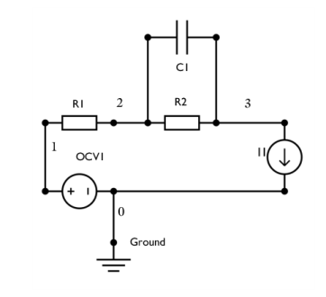
In the Model Builder window, under Component 1 (comp1)>Electrical Circuit (cir) click Resistor 1 (R1).
|
|
2
|
|
3
|
|
1
|
|
2
|
In the Settings window for Battery Open Circuit Voltage, locate the Capacity and Initial State-of-Charge section.
|
|
3
|
|
4
|
|
5
|
|
6
|
|
7
|
Browse to the model’s Application Libraries folder and double-click the file nimh_equivalent_circuit_battery_E_OCP_data.txt.
|
|
1
|
|
2
|
|
3
|
|
1
|
|
2
|
|
3
|
|
4
|
|
5
|
|
1
|
|
2
|
|
3
|
Click
|
|
1
|
|
2
|
|
3
|
|
4
|
|
1
|
|
2
|
|
3
|
|
4
|
|
1
|
|
2
|
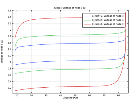
In the Settings window for Global, click Replace Expression in the upper-right corner of the y-Axis Data section. From the menu, choose Component 1 (comp1)>Electrical Circuit>Node voltages>cir.v_3 - Voltage at node 3 - V.
|
|
3
|
|
4
|
|
5
|
|
6
|
Select the Description check box.
|
|
7
|
In the associated text field, type Capacity.
|
|
8
|
|
9
|
|
1
|
|
2
|
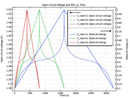
In the Settings window for 1D Plot Group, type Open Circuit Voltage and SOC vs. Time in the Label text field.
|
|
3
|
|
4
|
|
1
|
In the Model Builder window, expand the Open Circuit Voltage and SOC vs. Time node, then click Global 1.
|
|
2
|
In the Settings window for Global, click Replace Expression in the upper-right corner of the y-Axis Data section. From the menu, choose Component 1 (comp1)>Electrical Circuit>cir.OCV1.E_OCV - Open circuit voltage - V.
|
|
3
|
|
4
|
|
5
|
|
6
|
Click to expand the Coloring and Style section. Find the Line style subsection. From the Line list, choose Dashed.
|
|
1
|
|
2
|
In the Settings window for Global, click Replace Expression in the upper-right corner of the y-Axis Data section. From the menu, choose Component 1 (comp1)>Electrical Circuit>cir.OCV1.SOC - State-of-charge.
|
|
3
|
|
4
|
|
5
|
|
6
|
|
7
|