PDF

1D Isothermal Nickel-Cadmium Battery
Introduction
Nickel-Cadmium (NiCd) batteries are rechargeable batteries with nickel-hydroxide as positive electrode material, cadmium as negative electrode material, and hydroxide ions in an aqueous KOH electrolyte as charge carriers. Historically, they were used in many applications, for example those requiring high power. Today, mainly due to the toxicity of cadmium, their use is restricted. In the European Union, for example, they are only allowed in medical equipment and emergency systems and lighting. Lithium-ion and nickel-metal hydroxide batteries have replaced the NiCd battery in many applications.
The present model shows how a typical sealed NiCd battery cell can be described using the Battery with Binary Electrolyte interface.
Figure 1: Cross section of a NiCd battery showing the main electrochemical processes that occur during discharge.
The 1D isothermal model includes the following processes:
The model is based on a paper by De Vidts and White (Ref. 2) using data for a typical sealed NiCd battery (Ref. 1). In the paper, the authors also included a model for electron transport inside the positive electrode material. However, it was found that this contribution was negligible and it is therefore excluded in the present model.
Model Definition
This example models the battery cross section in 1D, which implies that edge effects in the length and height of the battery are neglected. The example uses the following domains:
In addition, an extra dimension description of the cylindrically symmetric particles in the positive electrode is included. These particles constitute long “wires”, with a central core of inactive support material. The thickness of the inactive core region is 1.5 μm, and the thickness of the active material surrounding it is 1.4 μm.
The electric potential in the electron conducting phase, , is calculated using a charge balance based on Ohm’s law, where the charge transfer reactions result in source or sink term. For the porous electrodes effective conductivities, σseff, are used that take porosity and tortuosity into account as given by the following expression:
where γ is the Bruggeman coefficient, which is set to 1.5 in this model, corresponding to a packed bed of spherical particles. Also, the diffusion coefficient for the electrolyte salt is corrected for the tortuosity and the porosity in this way.
The ionic charge balances and material balances are modeled according to the equations for a binary 1:1 electrolyte, with both the anion (OH-) and the solvent (H2O) participating in the electrode reactions (Ref. 2).
Fickian diffusion describes the transport in the cylindrical particles of the positive electrode. The diffusion equation is expressed in cylindrical coordinates for the material balance of protons in the particles.
Butler–Volmer electrode kinetics describes the local charge transfer current density in the electrodes. The Butler–Volmer expressions are introduced as source or sink terms in the charge balances and material balances.
Boundary Conditions
For the electronic current balance, a potential of 0 V is set on the negative electrode’s current collector/feeder boundary. At the positive electrode current collector/feeder, the current density is specified. The current density is set to a constant discharge current. The inner boundaries facing the separator are insulating for electric currents.
For the ionic charge balance in the electrolyte, the current collector/feeder boundaries are insulating. Insulating conditions also apply to the material balances.
At the particle surface in the local particle model, the material flux is determined by the local electrochemical reaction rate.
Material Properties
The material properties are those of a typical NiCd cell. The electrolyte is KOH, diluted in water to a 30% (wt) solution. The active electrode materials are cadmium for the negative electrode and a nickel oxide (Ni(OH)2) for the positive electrode.
The model uses constant values for the electrolyte conductivity, the electrolyte diffusivity, and the activity variation with concentration in the electrolyte.
The positive Ni electrode limits, and thus determines, the capacity of the battery cell. For this reason, the solid volume fraction of the Ni electrode is computed as
(1)
where Qcell is the cell capacity (74.16 C/cm2 of electrode), F is Faraday’s constant, cH, max is the maximum proton concentration in the positive material and lpositive is the thickness of the positive electrode (400 μm).
Results and Discussion
Simulations of both the discharge and charge behavior of the cell are performed. In both cases, three increasingly high C-rates of C/10, C/2.1, and C/0.7 are applied. The nominal charge/discharge current density, the 1C rate, is 206 A/m2.
Discharge Curves
Figure 2: Discharge curves for three C-rates.
Figure 2 shows discharge curves for the three C-rates. The overpotential of the positive electrode reaction increases with increasing C-rate, accounting for most of the difference in cell voltage at the initial time. At the end of discharge, the concentration of protons inside the positive electrode approaches the maximum value and the slopes of the voltage curves decrease drastically.
Charge Curves
Figure 3: Charge curves for the three C-rates.
Figure 3 shows charge curves for all three C-rates. Again, as for the discharge curves, the difference in initial potential is due mainly to the overpotential of the positive electrode reaction. However, as the cell approaches 100% state of charge (SOC), the oxygen side reaction takes up an increasing fraction of the applied current. The voltage then plateaus, and during overcharging all current goes toward oxygen evolution on the positive Ni electrode and reduction at the negative Cd electrode.
State of Charge During Charging
Figure 4 shows the hydration level of the positive Ni electrode, while Figure 5 shows the volume fraction of the negative Cd electrode, in both cases for charging. The x-axis shows the charge efficiency. Charging should reach completion at t = 1 for 100% charge efficiency. Charging causes protons to exit the positive electrode, and causes Cd hydroxide to be converted into metallic Cd. For this reason, decreasing hydration level and decreasing volume fraction both correspond to increasing SOC.
Figure 4: State of charge of the positive Ni electrode during charging at three different C-rates.
Both hydration level and volume fraction decrease in the same way during the initial part of charging, when the main electrode reactions consume almost all of the current. As charging approaches completion, after about t = 0.8, increasing C-rates are associated with decreased charge efficiency. Again, at higher C-rates, the oxygen side reaction consumes an increasing fraction of the charging current.
Figure 5: State of charge of the negative Cd electrode during charging at three different C-rates.
Notes About the COMSOL Implementation
Electrolyte Molar Mass
By default, the Battery with Binary Electrolyte interface assumes a binary aqueous KOH electrolyte, so the default values for molar masses on the main interface node do not need to be changed.
Proton Diffusion in Extra Dimension
Proton diffusion inside the positive Ni active material is modeled inside a cylindrically symmetric Extra Dimension. The following continuity equation, which accounts for the cylindrical symmetry, is applied for protons inside the active positive material:
(2)
Furthermore, at the exterior boundary of the Extra Dimension (the active material particle outer surface), the flux of cH is proportional to the current density of the main Ni electrode reaction. Both expressions are implemented in weak form.
The core of inactive support material is what necessitates the extra dimension description. If the Ni material particles had been assumed to be active throughout the whole radius, the Particle Properties of the Ni electrode could instead have been set to Intercalating Particles, and the diffusion of protons could have been set up in the associated Particle Intercalation child node.
Porous electrode electrical conductivity
The solid electrical conductivity of each of the two porous electrodes is on the order of 105 S/m. However, the electrolyte conductivity is significantly lower, and thus is the main factor limiting the rate of charge transport. This difference in conductivities makes convergence harder to achieve. Using an effective solid phase conductivity of 100 S/m facilitates convergence while having an insignificant effect on the results.
References
1. W.R. Scott and D.W. Rusta, Sealed-Cell Nickel Cadmium Battery Applications Manual, 1979.
2. P. De Vidts, and R.E. White, “Mathematical Modeling of a Nickel-Cadmium Cell: Proton Diffusion in the Nickel Electrode,” J. Electrochem. Soc., vol. 142, p. 1509, 1995.
Application Library path: Battery_Design_Module/Batteries,_General/nicd_battery_1d
Modeling Instructions
From the File menu, choose New.
New
In the New window, click  Model Wizard.
Model Wizard
1
In the Model Wizard window, click  1D.
2
In the Select Physics tree, select Electrochemistry>Batteries>Battery with Binary Electrolyte (batbe).
3
Click Add.
4
Click  Study.
5
In the Select Study tree, select Preset Studies for Selected Physics Interfaces>Time Dependent with Initialization.
6
Global Definitions
Define parameters for the model. These include general parameters (for example the geometry), parameters used for each electrode, for the electrode reactions, for initial values of the charging and discharging studies, and finally the different C-rates to use for charge and discharge.
General
1
In the Model Builder window, under Global Definitions right-click Parameters 1 and choose Rename.
2
In the Rename Parameters dialog box, type General in the New label text field.
3
4
In the Settings window for Parameters, locate the Parameters section.
5
Click  Load from File.
6
Cd Electrode
1
In the Home toolbar, click  Parameters and choose Add>Parameters.
2
Right-click Parameters 2 and choose Rename.
3
In the Rename Parameters dialog box, type Cd Electrode in the New label text field.
4
5
In the Settings window for Parameters, locate the Parameters section.
6
Click  Load from File.
7
Ni Electrode
1
In the Home toolbar, click  Parameters and choose Add>Parameters.
2
In the Model Builder window, right-click Parameters 3 and choose Rename.
3
In the Rename Parameters dialog box, type Ni Electrode in the New label text field.
4
5
In the Settings window for Parameters, locate the Parameters section.
6
Click  Load from File.
7
Electrode Reactions
1
In the Home toolbar, click  Parameters and choose Add>Parameters.
2
Right-click Parameters 4 and choose Rename.
3
In the Rename Parameters dialog box, type Electrode Reactions in the New label text field.
4
5
In the Settings window for Parameters, locate the Parameters section.
6
Click  Load from File.
7
Charge/Discharge Cases
1
In the Home toolbar, click  Parameters and choose Add>Parameters.
2
In the Model Builder window, right-click Parameters 5 and choose Rename.
3
In the Rename Parameters dialog box, type Charge/Discharge Cases in the New label text field.
4
5
In the Settings window for Parameters, locate the Parameters section.
6
7
In the Home toolbar, click  Parameter Case.
8
Right-click Case 1 and choose Rename.
9
In the Rename Case dialog box, type Discharge in the New label text field.
10
11
In the Home toolbar, click  Parameter Case.
12
In the Model Builder window, right-click Case 2 and choose Rename.
13
In the Rename Case dialog box, type Charge in the New label text field.
14
15
In the Settings window for Case, locate the Parameters section.
16
C-rate Cases
1
In the Home toolbar, click  Parameters and choose Add>Parameters.
2
In the Settings window for Parameters, type C-rate Cases in the Label text field.
3
Locate the Parameters section. In the table, enter the following settings:
4
In the Home toolbar, click  Parameter Case.
5
In the Settings window for Case, locate the Parameters section.
6
7
In the Home toolbar, click  Parameter Case.
8
In the Settings window for Case, locate the Parameters section.
9
10
In the Home toolbar, click  Parameter Case.
11
In the Settings window for Case, locate the Parameters section.
12
Define the cylindrical geometry of the electrode particles in the positive electrode in an Extra Dimension.
13
Click the  Show More Options button in the Model Builder toolbar.
14
In the Show More Options dialog box, select Physics>Extra Dimensions in the tree.
15
16
Add Component
In the Model Builder window, right-click Global Definitions and choose Extra Dimensions>1D Axisymmetric.
Extra Dimension: Positive Electrode
1
In the Model Builder window, under Global Definitions right-click Extra Dimension 1 (xdim1) and choose Rename.
2
In the Rename Extra Dimension dialog box, type Extra Dimension: Positive Electrode in the New label text field.
3
4
In the Settings window for Extra Dimension, locate the General section.
5
Find the Spatial frame coordinates subsection. In the table, enter the following settings:
Geometry 2
Interval 1 (i1)
1
In the Model Builder window, expand the Global Definitions>Extra Dimension: Positive Electrode (xdim1)>Definitions node.
2
Right-click Global Definitions>Extra Dimension: Positive Electrode (xdim1)>Geometry 2 and choose Interval.
The geometry of the positive electrode particles consists of an inner core of inactive substrate surrounded by active battery material.
3
In the Settings window for Interval, locate the Interval section.
4
From the Specify list, choose Interval lengths.
5
In the Left endpoint text field, type y_positive_substrate.
6
7
Click  Build Selected.
Define two integration operators to allow integration of variables in the extra dimension. These will be used later to compute the particle surface proton concentration as well as the average proton concentration inside the particle.
Definitions (xdim1)
Extra Dimension Surface Integral
1
In the Model Builder window, under Global Definitions>Extra Dimension: Positive Electrode (xdim1)>Definitions right-click Extra Dimensions and choose Integration over Extra Dimension.
2
In the Settings window for Integration over Extra Dimension, type Extra Dimension Surface Integral in the Label text field.
3
Locate the Operator Name section. In the Operator name text field, type xdsurfop.
4
Locate the Source Selection section. From the Geometric entity level list, choose Boundary.
5
6
Locate the Advanced section. Clear the Compute integral in revolved geometry check box.
Extra Dimension Domain Integral
1
Right-click Extra Dimensions and choose Integration over Extra Dimension.
2
In the Settings window for Integration over Extra Dimension, type Extra Dimension Domain Integral in the Label text field.
3
Locate the Operator Name section. In the Operator name text field, type xdintopDomain.
4
5
Locate the Advanced section. Clear the Compute integral in revolved geometry check box.
Make the mesh finer close to the left and right boundaries of the extra dimension.
Mesh 2
1
In the Model Builder window, under Global Definitions>Extra Dimension: Positive Electrode (xdim1) click Mesh 2.
2
In the Settings window for Mesh, locate the Mesh Settings section.
3
From the Sequence type list, choose User-controlled mesh.
Distribution 1
1
Right-click Global Definitions>Extra Dimension: Positive Electrode (xdim1)>Mesh 2 and choose Distribution.
2
3
In the Settings window for Distribution, locate the Distribution section.
4
From the Distribution type list, choose Predefined.
5
In the Number of elements text field, type 31.
6
In the Element ratio text field, type 0.1.
7
Click  Build All.
Next, define the geometry for the battery cell.
Geometry 1
Interval 1 (i1)
1
In the Model Builder window, expand the Component 1 (comp1)>Geometry 1 node.
2
Right-click Geometry 1 and choose Interval.
3
In the Settings window for Interval, locate the Interval section.
4
From the Specify list, choose Interval lengths.
5
6
Click  Build All Objects.
Define the connection between the battery cell geometry and the extra dimension used for the cylindrical battery particles.
Definitions (comp1)
Attached Dimensions 1
1
In the Model Builder window, expand the Component 1 (comp1)>Definitions node.
2
Right-click Component 1 (comp1)>Definitions>Extra Dimensions and choose Attached Dimensions.
3
In the Settings window for Attached Dimensions, locate the Geometric Entity Selection section.
4
From the Geometric entity level list, choose Domain.
5
6
Locate the Attached Dimensions section. Under Extra dimensions to attach, click  Add.
7
In the Add dialog box, select Extra Dimension: Positive Electrode (xdim1) in the Extra dimensions to attach list.
8
Define the variables needed for the SOC of the negative electrode, the SOC and diffusive flux of protons inside the positive electrode, and the surface and average proton concentration and SOC at the positive electrode.
Negative Electrode
1
In the Model Builder window, right-click Definitions and choose Variables.
2
In the Settings window for Variables, type Negative Electrode in the Label text field.
3
Locate the Geometric Entity Selection section. From the Geometric entity level list, choose Domain.
4
5
Locate the Variables section. In the table, enter the following settings:
Positive Electrode (Intra-particle)
1
Right-click Definitions and choose Variables.
2
Right-click Variables 2 and choose Rename.
3
In the Rename Variables dialog box, type Positive Electrode (Intra-particle) in the New label text field.
4
5
In the Settings window for Variables, locate the Geometric Entity Selection section.
6
From the Geometric entity level list, choose Domain.
7
8
From the Extra dimension attachment list, choose Attached Dimensions 1.
9
Locate the Variables section. In the table, enter the following settings:
Positive Electrode (Particle Surface)
1
In the Model Builder window, right-click Definitions and choose Variables.
2
In the Settings window for Variables, type Positive Electrode (Particle Surface) in the Label text field.
3
Locate the Geometric Entity Selection section. From the Geometric entity level list, choose Domain.
4
5
Locate the Variables section. In the table, enter the following settings:
At this point, all the entries are shown in yellow since further settings are needed to fully define the variables.
Define three operators: one for the positive electrode current collector, one for positive electrode averages, and one for negative electrode averages.
Integration Operator for Positive Electrode Current Collector
1
In the Definitions toolbar, click  Nonlocal Couplings and choose Integration.
2
Right-click Integration 1 (intop1) and choose Rename.
3
In the Rename Integration dialog box, type Integration Operator for Positive Electrode Current Collector in the New label text field.
4
5
In the Settings window for Integration, type intop_posCC in the Operator name text field.
6
Locate the Source Selection section. From the Geometric entity level list, choose Boundary.
7
Positive Electrode Average Operator
1
In the Definitions toolbar, click  Nonlocal Couplings and choose Average.
2
In the Settings window for Average, type Positive Electrode Average Operator in the Label text field.
3
In the Operator name text field, type ave_pos.
4
Negative Electrode Average Operator
1
In the Definitions toolbar, click  Nonlocal Couplings and choose Average.
2
In the Settings window for Average, type Negative Electrode Average Operator in the Label text field.
3
In the Operator name text field, type ave_neg.
4
The next step is to set up the description of the chemical processes inside the battery. Begin with the Battery with Binary Electrolyte interface.
Battery with Binary Electrolyte (batbe)
By default, the Battery with Binary Electrolyte interface assumes a KOH binary electrolyte, so the default values for the Species section will be kept. However, properties for the KOH electrolyte for the porous electrodes and separator need to be specified. These are available in the Material Library.
Add Material
1
In the Home toolbar, click  Add Material to open the Add Material window.
2
Go to the Add Material window.
3
In the tree, select Battery>Electrolytes>KOH (Liquid binary electrolyte).
4
Click Add to Component in the window toolbar.
5
In the Home toolbar, click  Add Material to close the Add Material window.
Battery with Binary Electrolyte (batbe)
Initial Values 1
1
In the Model Builder window, under Component 1 (comp1)>Battery with Binary Electrolyte (batbe) click Initial Values 1.
2
In the Settings window for Initial Values, locate the Initial Values section.
3
In the cl text field, type cl_init.
Continue by setting up the description for the Ni (positive) electrode.
Porous Electrode: Ni (Positive)
1
In the Physics toolbar, click  Domains and choose Porous Electrode.
2
Right-click Porous Electrode 1 and choose Rename.
3
In the Rename Porous Electrode dialog box, type Porous Electrode: Ni (Positive) in the New label text field.
4
5
6
In the Settings window for Porous Electrode, locate the Electrode Properties section.
7
From the σs list, choose User defined. In the associated text field, type sigma_electrode.
8
Locate the Particle Properties section. From the list, choose Nonintercalating particles.
9
Locate the Porous Matrix Properties section. In the εs text field, type epss.
10
In the εl text field, type epsilon0_P-epss.
11
Locate the Effective Transport Parameter Correction section. From the Electrical conductivity list, choose No correction.
Set up the intercalaction process for protons at the Ni electrode.
Porous Electrode Reaction: NiOOH + H2O + e- <=> Ni(OH)2 + OH-
1
In the Model Builder window, expand the Porous Electrode: Ni (Positive) node.
2
Right-click Porous Electrode Reaction 1 and choose Rename.
3
In the Rename Porous Electrode Reaction dialog box, type Porous Electrode Reaction: NiOOH + H2O + e- <=> Ni(OH)2 + OH- in the New label text field.
4
5
In the Settings window for Porous Electrode Reaction, locate the Equilibrium Potential section.
6
From the Eeq list, choose Nernst equation.
7
In the Eeq,ref(T) text field, type E_ref_pos.
8
In the CR text field, type (cl/c_ref)*(cH_surf/c_H_ref).
9
In the CO text field, type (c_H_max-cH_surf)/(c_H_max-c_H_ref).
10
Locate the Electrode Kinetics section. From the Kinetics expression type list, choose Butler-Volmer.
11
From the Exchange current density type list, choose From Nernst Equation.
12
In the i0,ref(T) text field, type i0_1_ref.
13
In the αa text field, type alpha_a_1.
14
Locate the Active Specific Surface Area section. From the Active specific surface area list, choose User defined. In the av text field, type a_Ni.
15
Click to expand the Heat of Reaction section. From the dEeq/dT list, choose User defined.
Add the OER/ORR reaction on the Ni electrode. The mass transport of oxygen inside the battery cell will be set up later.
Porous Electrode: Ni (Positive)
In the Model Builder window, click Porous Electrode: Ni (Positive).
Porous Electrode Reaction: 1/2 O2 + H2O + 2e- <=> 2 OH-
1
In the Physics toolbar, click  Attributes and choose Porous Electrode Reaction.
2
Right-click Porous Electrode Reaction 2 and choose Rename.
3
In the Rename Porous Electrode Reaction dialog box, type Porous Electrode Reaction: 1/2 O2 + H2O + 2e- <=> 2 OH- in the New label text field.
4
5
In the Settings window for Porous Electrode Reaction, locate the Equilibrium Potential section.
6
From the Eeq list, choose Nernst equation.
7
In the Eeq,ref(T) text field, type E_ref_OER.
8
In the CR text field, type 1.
9
In the CO text field, type c_O2/c_O2_ref.
10
Locate the Electrode Kinetics section. From the Kinetics expression type list, choose Butler-Volmer.
11
From the Exchange current density type list, choose From Nernst Equation.
Use a max() operator to numerically stabilize the kinetics expression.
12
In the i0,ref(T) text field, type i0_2_ref*max(cl/c_ref,1e-20)^2.
13
In the αa text field, type alpha_a_2.
14
Locate the Active Specific Surface Area section. From the Active specific surface area list, choose User defined. In the av text field, type a_Ni.
15
Locate the Stoichiometric Coefficients section. In the n text field, type 4.
16
Locate the Heat of Reaction section. From the dEeq/dT list, choose User defined. Set up the diffusion of protons inside the positive electrode. Add one weak expression for the diffusive flux and one weak expression for the boundary flux due to the NiOOH/Ni(OH)2 electrode reaction.
17
Click the  Show More Options button in the Model Builder toolbar.
18
In the Show More Options dialog box, select Physics>Stabilization in the tree.
19
20
In the tree, select Physics>Stabilization.
21
22
In the tree, select Physics>Equation-Based Contributions.
23
In the tree, select the check box for the node Physics>Equation-Based Contributions.
24
H+ Diffusion Inside Positive Electrode
1
In the Physics toolbar, click  Domains and choose Weak Contribution.
2
In the Settings window for Weak Contribution, type H+ Diffusion Inside Positive Electrode in the Label text field.
3
4
Locate the Domain Selection section. From the Extra dimension attachment list, choose Attached Dimensions 1.
5
Select the  Activate Selection toggle button.
6
7
Locate the Weak Contribution section. In the Weak expression text field, type 2*pi*rxd*(particle_diffusive_flux*test(cHrxd)-cHt*test(cH)).
Intra-particle H+ Concentration
1
In the Physics toolbar, click  Attributes and choose Auxiliary Dependent Variable.
2
Right-click Auxiliary Dependent Variable 1 and choose Rename.
3
In the Rename Auxiliary Dependent Variable dialog box, type Intra-particle H+ Concentration in the New label text field.
4
5
In the Settings window for Auxiliary Dependent Variable, locate the Domain Selection section.
6
From the Extra dimension attachment list, choose Attached Dimensions 1.
7
Select the  Activate Selection toggle button.
8
9
Locate the Auxiliary Dependent Variable section. In the Field variable name text field, type cH.
10
In the Initial value text field, type c_H_init.
Boundary Condition for Concentration at Particle Outer Surface
1
In the Physics toolbar, click  Domains and choose Weak Contribution.
2
In the Settings window for Weak Contribution, type Boundary Condition for Concentration at Particle Outer Surface in the Label text field.
3
4
Locate the Domain Selection section. From the Extra dimension attachment list, choose Attached Dimensions 1.
5
From the Geometric entity level list, choose Boundary.
6
7
Locate the Weak Contribution section. In the Weak expression text field, type -2*batbe.pce1.per1.iloc*test(cH)*pi*rxd/(1[m]*F_const).
Boundary Condition for Concentration at Particle Outer Surface, H+ Diffusion Inside Positive Electrode
1
In the Model Builder window, under Component 1 (comp1)>Battery with Binary Electrolyte (batbe), Ctrl-click to select H+ Diffusion Inside Positive Electrode and Boundary Condition for Concentration at Particle Outer Surface.
2
Intra-particle Diffusion of H+
1
In the Model Builder window, right-click Group 1 and choose Rename.
2
In the Rename Group dialog box, type Intra-particle Diffusion of H+ in the New label text field.
3
Continue by defining the separator and the Cd (negative) electrode.
Separator 1
1
In the Physics toolbar, click  Domains and choose Separator.
2
3
In the Settings window for Separator, locate the Porous Matrix Properties section.
4
In the εl text field, type epsilon_2.
Porous Electrode: Cd (Negative)
1
In the Physics toolbar, click  Domains and choose Porous Electrode.
2
In the Settings window for Porous Electrode, type Porous Electrode: Cd (Negative) in the Label text field.
3
4
Locate the Electrode Properties section. From the σs list, choose User defined. In the associated text field, type sigma_electrode.
5
Locate the Particle Properties section. From the list, choose Nonintercalating particles.
6
Locate the Porous Matrix Properties section. In the εs text field, type 1-epsilon_3_init.
7
In the εl text field, type epsilon_3_init.
8
Locate the Effective Transport Parameter Correction section. From the Electrical conductivity list, choose No correction.
9
Click to expand the Dissolving-Depositing Species section. Click  Add.
10
11
12
Porous Electrode Reaction: Cd + 2 OH- <=> Cd(OH)2 + 2e-
1
In the Model Builder window, expand the Porous Electrode: Cd (Negative) node.
2
Right-click Porous Electrode Reaction 1 and choose Rename.
3
In the Rename Porous Electrode Reaction dialog box, type Porous Electrode Reaction: Cd + 2 OH- <=> Cd(OH)2 + 2e- in the New label text field.
4
5
In the Settings window for Porous Electrode Reaction, locate the Equilibrium Potential section.
6
From the Eeq list, choose Nernst equation.
7
In the Eeq,ref(T) text field, type E_ref_neg.
8
In the CR text field, type (cl/c_ref)^2.
9
Locate the Electrode Kinetics section. From the Kinetics expression type list, choose Butler-Volmer.
10
From the Exchange current density type list, choose From Nernst Equation.
11
In the i0,ref(T) text field, type theta_N*i0_3_ref.
12
In the αa text field, type alpha_a_3.
13
Locate the Active Specific Surface Area section. From the Active specific surface area list, choose User defined. In the av text field, type a_Cd.
14
Locate the Stoichiometric Coefficients section. In the n text field, type 2.
15
In the Stoichiometric coefficients for dissolving-depositing species: table, enter the following settings:
16
Locate the Heat of Reaction section. From the dEeq/dT list, choose User defined.
The oxygen reduction reaction is mass-transport limited at the Cd electrode. Model it using an Internal Electrode Surface, with the local current density being given by an oxygen flux at the Cd electrode. In turn, the flux will be obtained from a Transport of Diluted Species interface, where the diffusion of oxygen in the battery is also modeled.
Oxygen Recombination at Cd Electrode
1
In the Physics toolbar, click  Boundaries and choose Internal Electrode Surface.
2
In the Settings window for Internal Electrode Surface, type Oxygen Recombination at Cd Electrode in the Label text field.
3
Electrode Reaction: 1/2 O2 + H2O + 2e- <=> 2 OH-
1
In the Model Builder window, expand the Oxygen Recombination at Cd Electrode node.
2
Right-click Electrode Reaction 1 and choose Rename.
3
In the Rename Electrode Reaction dialog box, type Electrode Reaction: 1/2 O2 + H2O + 2e- <=> 2 OH- in the New label text field.
4
5
In the Settings window for Electrode Reaction, locate the Equilibrium Potential section.
6
From the Eeq list, choose User defined. Locate the Electrode Kinetics section. From the iloc,expr list, choose User defined. In the associated text field, type tds.tflux_c_O2x*4*F_const.
7
Click to expand the Heat of Reaction section. From the dEeq/dT list, choose User defined.
Define the boundary conditions for the battery cell
Electric Ground 1
1
In the Physics toolbar, click  Boundaries and choose Electric Ground.
2
Electrode Current 1
1
In the Physics toolbar, click  Boundaries and choose Electrode Current.
2
3
In the Settings window for Electrode Current, locate the Electrode Current section.
4
From the list, choose Average current density.
5
In the is,average text field, type sign*i_app.
Set up the description of the oxygen transport and reaction.
Add Physics
1
In the Physics toolbar, click  Add Physics to open the Add Physics window.
2
Go to the Add Physics window.
3
In the tree, select Chemical Species Transport>Transport of Diluted Species (tds).
4
Click Add to Component 1 in the window toolbar.
5
In the Physics toolbar, click  Add Physics to close the Add Physics window.
Transport of Diluted Species (tds)
1
In the Settings window for Transport of Diluted Species, locate the Transport Mechanisms section.
2
Clear the Convection check box.
3
Select the Mass transfer in porous media check box.
4
Click to expand the Dependent Variables section. In the Concentrations table, enter the following settings:
5
Transport Properties 1
1
In the Model Builder window, under Component 1 (comp1)>Transport of Diluted Species (tds) click Transport Properties 1.
2
In the Settings window for Transport Properties, locate the Diffusion section.
3
In the DcO2 text field, type D_O2.
Initial Values 1
1
In the Model Builder window, click Initial Values 1.
2
In the Settings window for Initial Values, locate the Initial Values section.
3
In the cO2 text field, type c_O2_init.
Porous Electrode Coupling: Positive Electrode
1
In the Physics toolbar, click  Domains and choose Porous Electrode Coupling.
2
In the Settings window for Porous Electrode Coupling, type Porous Electrode Coupling: Positive Electrode in the Label text field.
3
Reaction Coefficients 1
1
In the Model Builder window, expand the Porous Electrode Coupling: Positive Electrode node, then click Reaction Coefficients 1.
2
In the Settings window for Reaction Coefficients, locate the Model Inputs section.
3
From the iv list, choose Local current source, Porous Electrode Reaction: 1/2 O2 + H2O + 2e- <=> 2 OH- (batbe/pce1/per2).
4
Locate the Stoichiometric Coefficients section. In the n text field, type 4.
5
In the νcO2 text field, type -1.
Oxygen Recombination at Cd Electrode
1
In the Physics toolbar, click  Boundaries and choose Concentration.
2
In the Settings window for Concentration, type Oxygen Recombination at Cd Electrode in the Label text field.
3
4
Locate the Concentration section. Select the Species c_O2 check box.
Initial Values 2
1
In the Physics toolbar, click  Domains and choose Initial Values.
Add a suitable initial value for the oxygen concentration in the separator.
2
3
In the Settings window for Initial Values, locate the Initial Values section.
4
In the cO2 text field, type c_O2_init*((x-l_neg)/l_sep).
The battery model, including the oxygen transport and reaction, has now been set up. Now, configure the study to simulate both discharging, and charging, of the battery.
Discharge and Charge
1
In the Model Builder window, right-click Study 1 and choose Rename.
2
In the Rename Study dialog box, type Discharge and Charge in the New label text field.
3
Parametric Sweep
1
In the Study toolbar, click  Parametric Sweep.
2
In the Settings window for Parametric Sweep, locate the Study Settings section.
3
From the Sweep type list, choose Parameter switch.
4
5
6
7
Current Distribution Initialization: Primary
1
In the Model Builder window, click Step 1: Current Distribution Initialization.
2
In the Settings window for Current Distribution Initialization, type Current Distribution Initialization: Primary in the Label text field.
3
Locate the Physics and Variables Selection section. In the table, clear the Solve for check box for Transport of Diluted Species (tds).
Current Distribution Initialization: Secondary
1
In the Study toolbar, click  Study Steps and choose Other>Current Distribution Initialization.
2
Right-click Discharge and Charge>Step 3: Current Distribution Initialization 2 and choose Move Up.
3
In the Settings window for Current Distribution Initialization, type Current Distribution Initialization: Secondary in the Label text field.
4
Locate the Physics and Variables Selection section. In the table, clear the Solve for check box for Transport of Diluted Species (tds).
Use an additional Current Distribution Initialization step, solving for a secondary current distribution, to improve the initial guess further.
5
Locate the Study Settings section. From the Current distribution type list, choose Secondary.
Step 3: Time Dependent
1
In the Model Builder window, click Step 3: Time Dependent.
2
In the Settings window for Time Dependent, locate the Study Settings section.
3
From the Time unit list, choose h.
4
In the Output times text field, type range(0,t_charge_limit/100,t_charge_limit).
Before starting to solve, to make convergence easier to achieve, manually set the scaling for the oxygen concentration, and the proton concentration in the extra dimension. The corresponding reference concentrations are suitable values for scaling.
Solution 1 (sol1)
1
In the Study toolbar, click  Show Default Solver.
2
In the Model Builder window, expand the Solution 1 (sol1) node.
3
In the Model Builder window, expand the Discharge and Charge>Solver Configurations>Solution 1 (sol1)>Dependent Variables 3 node, then click Concentration (comp1.c_O2).
4
In the Settings window for Field, locate the Scaling section.
5
From the Method list, choose Manual.
6
In the Scale text field, type c_O2_ref.
7
In the Model Builder window, click Auxiliary dependent variable cH (comp1.cH).
8
In the Settings window for Field, click to collapse the Scaling section.
9
Click to expand the Scaling section. From the Method list, choose Manual.
10
In the Scale text field, type c_H_ref.
Additionally, set up two Stop conditions, signaling the solver to stop if the cell voltage gets below 0.8 V or above 1.6 V.
11
In the Model Builder window, right-click Time-Dependent Solver 1 and choose Stop Condition.
12
In the Settings window for Stop Condition, locate the Stop Expressions section.
13
14
15
16
Store the solution just after the stop condition to include the data at the lowest and highest voltages reached in the results.
17
Locate the Output at Stop section. From the Add solution list, choose Step after stop.
Now, run the study for discharge and charge of the battery.
18
In the Study toolbar, click  Compute.
Results
Discharge: Boundary Electrode Potential with Respect to Ground (batbe)
Plot the cell voltage for discharge at the three different C-rates.
1
Right-click Results>Boundary Electrode Potential with Respect to Ground (batbe) and choose Rename.
2
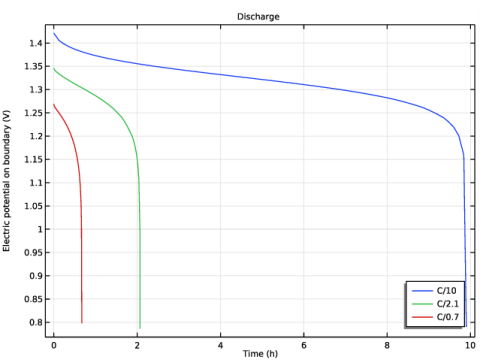
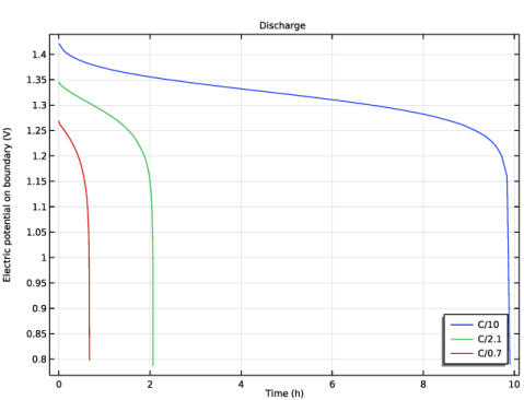
In the Rename 1D Plot Group dialog box, type Discharge: Boundary Electrode Potential with Respect to Ground (batbe) in the New label text field.
3
4
In the Settings window for 1D Plot Group, locate the Data section.
5
From the Parameter selection (c_H_init, epsilon_3_init, sign, C_rate) list, choose From list.
6
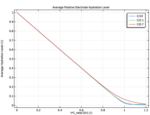
In the Parameter values list, choose 1: c_H_init=104.2, epsilon_3_init=0.6365, sign=-1, C_rate=0.1, 2: c_H_init=104.2, epsilon_3_init=0.6365, sign=-1, C_rate=0.47619, and 3: c_H_init=104.2, epsilon_3_init=0.6365, sign=-1, C_rate=1.4286.
7
In the Discharge: Boundary Electrode Potential with Respect to Ground (batbe) toolbar, click  Plot.
Global 1
1
In the Model Builder window, expand the Discharge: Boundary Electrode Potential with Respect to Ground (batbe) node, then click Global 1.
2
In the Settings window for Global, locate the x-Axis Data section.
3
From the Parameter list, choose Expression.
4
In the Expression text field, type t.
5
From the Unit list, choose h.
6
Click to expand the Legends section. From the Legends list, choose Manual.
7
Discharge: Boundary Electrode Potential with Respect to Ground (batbe)
1
In the Model Builder window, click Discharge: Boundary Electrode Potential with Respect to Ground (batbe).
2
In the Settings window for 1D Plot Group, click to expand the Title section.
3
From the Title type list, choose Manual.
4
In the Title text area, type Discharge.
5
Locate the Legend section. From the Position list, choose Lower right.
6
In the Discharge: Boundary Electrode Potential with Respect to Ground (batbe) toolbar, click  Plot.
Plot the cell voltage for charging. Then, plot the average positive electrode hydration level (SOC) and the average negative electrode volume fraction (SOC).
Charge: Boundary Electrode Potential with Respect to Ground (batbe)
1
Right-click Discharge: Boundary Electrode Potential with Respect to Ground (batbe) and choose Duplicate.
2
Right-click Discharge: Boundary Electrode Potential with Respect to Ground (batbe) 1 and choose Rename.
3
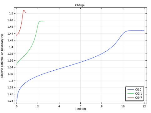
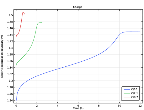
In the Rename 1D Plot Group dialog box, type Charge: Boundary Electrode Potential with Respect to Ground (batbe) in the New label text field.
4
5
In the Settings window for 1D Plot Group, locate the Data section.
6
In the Parameter values list, choose 4: c_H_init=52098, epsilon_3_init=0.46587, sign=1, C_rate=0.1, 5: c_H_init=52098, epsilon_3_init=0.46587, sign=1, C_rate=0.47619, and 6: c_H_init=52098, epsilon_3_init=0.46587, sign=1, C_rate=1.4286.
7
Locate the Title section. In the Title text area, type Charge.
8
In the Charge: Boundary Electrode Potential with Respect to Ground (batbe) toolbar, click  Plot.
Charge: Average Positive Electrode Hydration Level
1
In the Home toolbar, click  Add Plot Group and choose 1D Plot Group.
2
Right-click 1D Plot Group 7 and choose Rename.
3
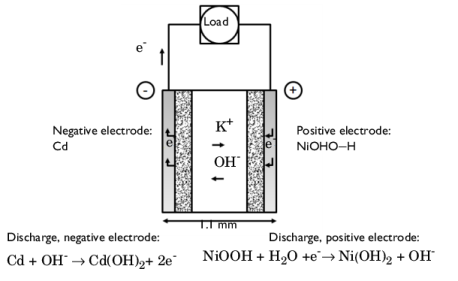
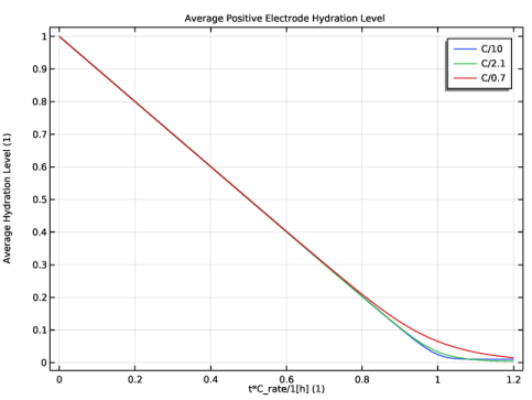
In the Rename 1D Plot Group dialog box, type Charge: Average Positive Electrode Hydration Level in the New label text field.
4
5
In the Settings window for 1D Plot Group, locate the Data section.
6
From the Dataset list, choose Discharge and Charge/Parametric Solutions 1 (sol4).
7
From the Parameter selection (c_H_init, epsilon_3_init, sign, C_rate) list, choose From list.
8
In the Parameter values list, choose 4: c_H_init=52098, epsilon_3_init=0.46587, sign=1, C_rate=0.1, 5: c_H_init=52098, epsilon_3_init=0.46587, sign=1, C_rate=0.47619, and 6: c_H_init=52098, epsilon_3_init=0.46587, sign=1, C_rate=1.4286.
9
Locate the Title section. From the Title type list, choose Manual.
10
In the Title text area, type Average Positive Electrode Hydration Level.
Global 1
1
Right-click Charge: Average Positive Electrode Hydration Level and choose Global.
2
In the Settings window for Global, locate the y-Axis Data section.
3
4
Locate the x-Axis Data section. From the Parameter list, choose Expression.
Normalize the time by the C-rate to enable comparing hydration levels for increasing C-rates.
5
In the Expression text field, type t*C_rate/1[h].
6
Locate the Legends section. From the Legends list, choose Manual.
7
8
In the Charge: Average Positive Electrode Hydration Level toolbar, click  Plot.
Charge: Average Negative Electrode Volume Fraction
1
In the Home toolbar, click  Add Plot Group and choose 1D Plot Group.
2
Right-click 1D Plot Group 8 and choose Rename.
3
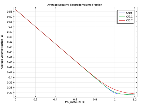
In the Rename 1D Plot Group dialog box, type Charge: Average Negative Electrode Volume Fraction in the New label text field.
4
5
In the Settings window for 1D Plot Group, locate the Data section.
6
From the Dataset list, choose Discharge and Charge/Parametric Solutions 1 (sol4).
7
From the Parameter selection (c_H_init, epsilon_3_init, sign, C_rate) list, choose From list.
8
In the Parameter values list, choose 4: c_H_init=52098, epsilon_3_init=0.46587, sign=1, C_rate=0.1, 5: c_H_init=52098, epsilon_3_init=0.46587, sign=1, C_rate=0.47619, and 6: c_H_init=52098, epsilon_3_init=0.46587, sign=1, C_rate=1.4286.
9
In the Charge: Average Negative Electrode Volume Fraction toolbar, click  Plot.
10
Locate the Title section. From the Title type list, choose Manual.
11
In the Title text area, type Average Negative Electrode Volume Fraction.
Global 1
1
Right-click Charge: Average Negative Electrode Volume Fraction and choose Global.
2
In the Settings window for Global, locate the y-Axis Data section.
3
4
Locate the x-Axis Data section. From the Parameter list, choose Expression.
5
In the Expression text field, type t*C_rate/1[h].
6
Locate the Legends section. From the Legends list, choose Manual.
7
8
In the Charge: Average Negative Electrode Volume Fraction toolbar, click  Plot.