PDF

Vibrating Particle in Water
Introduction
This is a model of a small particle oscillating in water, see Figure 1. It validates the numerical solution of the system of thermoviscous acoustics equations by comparison with an analytical solution given in Ref. 1. The Thermoviscous Acoustics, Frequency Domain interface is used for modeling the propagation of acoustic waves in small devices, where it is important to include losses in a detailed way. This is useful when modeling acoustics and vibrations in, for example, microphones, hearing aids, or MEMS devices. The interface provides a detailed way of solving the equations governing the propagation of acoustic waves in any fluid, including thermal conduction and viscous damping.
Figure 1: Sketch of the particle oscillating along the axis.
Acoustic waves are compressible waves and in the framework of the Thermoviscous Acoustics interface, a linearized equation of state is set up. This constitutive equation relates the acoustic variations in pressure p, density ρ, and temperature T through the expression
where ρ0 is the equilibrium density, βT is the isothermal compressibility, and αp is the coefficient of thermal expansion. The model shows a small sphere of radius 1 mm which is oscillating along the polar axis at 50 kHz. The sphere is modeled in 2D axisymmetry.
Note: Details about the governing equations are found in the theory section of the thermoviscous acoustics physics interface documentation. See File>Help>Documentation and search or open the Acoustics Module User’s Guide to the thermoviscous acoustics theory.
Model Definition
The model is set up in a 2D axisymmetric geometry; that is, the spatial coordinates are the radius, r, and the height, z. The spherical particle of the radius as vibrates along the z-axis with the velocity U0 = U0ez.
The analytical solution is obtained from the Helmholtz decomposition of the acoustic particle velocity
The velocity potential, , far from the sphere is defined as (Ref. 1)
(1)
where k is the wave number, R = (r + z)1/2, and b = kas. This yields the acoustic pressure
In this model, the adiabatic formulation of the system of thermoiviscous acoustics equations is solved. This formulation is appropriate because the thermal losses play a minor role in water compared to the viscous losses.
Since the acoustic waves radiated from the particle propagate in the free space, the computational domain used in the model should be truncated in a way that ensures wave propagation without reflections from the outer boundary. This is done in the model by surrounding the computational domain by a perfectly matched layer (PML).
Results and Discussion
The acoustic pressure variations and the instantaneous acoustic particle velocity in the physical domain are plotted in Figure 2 and in Figure 3. Figure 4 shows the pressure variations along the cut line directed from the particle top at the angle of 45° to the z-axis. The blue solid line and the green dotted line correspond to the numerical and the analytical solutions, respectively. The results match well except for the area near the particle. This is explained by the fact that Equation 1 is an asymptotic expression that is invalid near the particle. The exact expressions for and B can be found in Ref. 1.
Figure 2: Pressure variations in the water outside the small vibrating particle.
Figure 3: Instantaneous acoustic particle velocity in the water outside the small vibrating particle.
Figure 4: Pressure variation along the cut line: numerical and analytical solutions.
References
1. S. Temkin, Elements of Acoustics, Acoustical Society of America, 2001.
Application Library path: Acoustics_Module/Tutorials,_Thermoviscous_Acoustics/vibrating_particle_water
Modeling Instructions
From the File menu, choose New.
New
In the New window, click  Model Wizard.
Model Wizard
1
In the Model Wizard window, click  2D Axisymmetric.
2
In the Select Physics tree, select Acoustics>Thermoviscous Acoustics>Thermoviscous Acoustics, Frequency Domain (ta).
3
Click Add.
4
Click  Study.
5
In the Select Study tree, select General Studies>Frequency Domain.
6
Load the parameters from the file vibrating_particle_water_parameters.txt.
Global Definitions
Parameters 1
1
In the Model Builder window, under Global Definitions click Parameters 1.
2
In the Settings window for Parameters, locate the Parameters section.
3
Click  Load from File.
4
Geometry 1
Circle 1 (c1)
1
In the Geometry toolbar, click  Circle.
The thermal losses only play a minor role in water and can therefore be neglected by solving the system of thermoviscous equations in adiabatic formulation.
2
In the Settings window for Circle, locate the Size and Shape section.
3
In the Radius text field, type a_s.
4
Click  Build Selected.
Circle 2 (c2)
1
Right-click Circle 1 (c1) and choose Duplicate.
2
In the Settings window for Circle, locate the Size and Shape section.
3
In the Radius text field, type a_tot.
4
Click to expand the Layers section. In the table, enter the following settings:
Difference 1 (dif1)
1
In the Geometry toolbar, click  Booleans and Partitions and choose Difference.
2
3
In the Settings window for Difference, locate the Difference section.
4
Find the Objects to subtract subsection. Select the  Activate Selection toggle button.
5
6
Click  Build All Objects.
Definitions
Variables 1
1
In the Model Builder window, under Component 1 (comp1) right-click Definitions and choose Variables.
2
In the Settings window for Variables, locate the Variables section.
3
Perfectly Matched Layer 1 (pml1)
1
In the Definitions toolbar, click  Perfectly Matched Layer.
2
3
In the Settings window for Perfectly Matched Layer, locate the Scaling section.
4
From the Coordinate stretching type list, choose Rational.
Add Material
1
In the Home toolbar, click  Add Material to open the Add Material window.
2
Go to the Add Material window.
3
In the tree, select Built-in>Water, liquid.
4
Click Add to Component in the window toolbar.
5
In the Home toolbar, click  Add Material to close the Add Material window.
Thermoviscous Acoustics, Frequency Domain (ta)
1
In the Model Builder window, under Component 1 (comp1) click Thermoviscous Acoustics, Frequency Domain (ta).
2
In the Settings window for Thermoviscous Acoustics, Frequency Domain, locate the Sound Pressure Level Settings section.
3
From the Reference pressure for the sound pressure level list, choose Use reference pressure for water.
4
Locate the Typical Wave Speed for Perfectly Matched Layers section. In the cref text field, type c0.
5
Locate the Thermoviscous Acoustics Equation Settings section. Select the Adiabatic formulation check box.
Velocity 1
1
In the Physics toolbar, click  Boundaries and choose Velocity.
2
3
In the Settings window for Velocity, locate the Velocity section.
4
Select the Prescribed in r direction check box.
5
Select the Prescribed in z direction check box.
6
In the u0z text field, type U0.
Now, proceed and set up the mesh.
Mesh 1
1
In the Model Builder window, under Component 1 (comp1) click Mesh 1.
2
In the Settings window for Mesh, locate the Mesh Settings section.
3
From the Sequence type list, choose User-controlled mesh.
Size
1
In the Model Builder window, under Component 1 (comp1)>Mesh 1 click Size.
2
In the Settings window for Size, locate the Element Size section.
3
Click the Custom button.
4
Locate the Element Size Parameters section. In the Maximum element size text field, type lam0/10.
Free Triangular 1
1
In the Model Builder window, click Free Triangular 1.
2
In the Settings window for Free Triangular, locate the Domain Selection section.
3
From the Geometric entity level list, choose Domain.
4
Size 1
1
Right-click Free Triangular 1 and choose Size.
2
In the Settings window for Size, locate the Geometric Entity Selection section.
3
From the Geometric entity level list, choose Boundary.
4
5
Locate the Element Size section. Click the Custom button.
6
Locate the Element Size Parameters section. Select the Curvature factor check box.
7
Add Boundary Layers around the oscillating sphere to resolve the viscous penetration depth dvisc.
Boundary Layers 1
1
In the Mesh toolbar, click  Boundary Layers.
2
In the Settings window for Boundary Layers, locate the Domain Selection section.
3
From the Geometric entity level list, choose Domain.
4
Boundary Layer Properties
1
In the Model Builder window, click Boundary Layer Properties.
2
3
In the Settings window for Boundary Layer Properties, locate the Boundary Layer Properties section.
4
In the Number of boundary layers text field, type 10.
5
In the Boundary layer stretching factor text field, type 1.5.
6
From the Thickness of first layer list, choose Manual.
7
In the Thickness text field, type 0.3*dvisc.
Mapped 1
In the Mesh toolbar, click  Mapped.
Distribution 1
1
Right-click Mapped 1 and choose Distribution.
2
3
In the Settings window for Distribution, locate the Distribution section.
4
In the Number of elements text field, type 8.
5
Click  Build All.
Study 1
Step 1: Frequency Domain
1
In the Model Builder window, under Study 1 click Step 1: Frequency Domain.
2
In the Settings window for Frequency Domain, locate the Study Settings section.
3
In the Frequencies text field, type f0.
4
In the Home toolbar, click  Compute.
Results
Acoustic Pressure (ta)
1
In the Settings window for 2D Plot Group, click to expand the Title section.
2
From the Title type list, choose Manual.
3
In the Title text area, type Total acoustic pressure (Pa).
4
Locate the Color Legend section. Select the Show units check box.
Selection 1
1
In the Model Builder window, expand the Acoustic Pressure (ta) node.
2
Right-click Surface and choose Selection.
3
4
In the Acoustic Pressure (ta) toolbar, click  Plot.
The figure should look like the one in Figure 2.
Acoustic Velocity (ta)
1
In the Model Builder window, click Acoustic Velocity (ta).
2
In the Settings window for 2D Plot Group, locate the Title section.
3
From the Title type list, choose Manual.
4
In the Title text area, type Instantaneous Local Velocity (dB).
5
Locate the Color Legend section. Select the Show units check box.
The acoustic velocity quickly fades away as the distance from the particle grows. Use the logarithmic scale with the reference value U0 for better visualization of the velocity profile.
Surface
1
In the Model Builder window, expand the Acoustic Velocity (ta) node, then click Surface.
2
In the Settings window for Surface, locate the Expression section.
3
In the Expression text field, type 10*log10(abs(ta.v_inst/U0))[dB].
Selection 1
1
Right-click Surface and choose Selection.
2
3
In the Acoustic Velocity (ta) toolbar, click  Plot.
The figure should look like the one in Figure 3.
Create a Cut Line 2D dataset to compare the numerical and the analytical solutions.
Cut Line 2D 1
1
In the Results toolbar, click  Cut Line 2D.
2
In the Settings window for Cut Line 2D, locate the Line Data section.
3
In row Point 2, set R to a_ta/sqrt(2).
4
In row Point 2, set Z to a_ta/sqrt(2).
Total Acoustic Pressure
1
In the Results toolbar, click  1D Plot Group.
2
In the Settings window for 1D Plot Group, type Total Acoustic Pressure in the Label text field.
3
Locate the Data section. From the Dataset list, choose Cut Line 2D 1.
4
Click to expand the Title section. From the Title type list, choose Manual.
5
In the Title text area, type Acoustic Pressure: Model vs. Analytical.
6
Locate the Plot Settings section. Select the y-axis label check box.
7
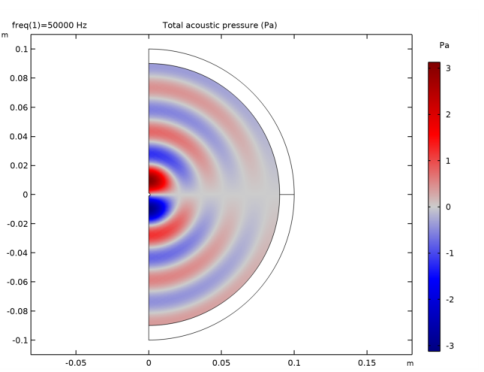
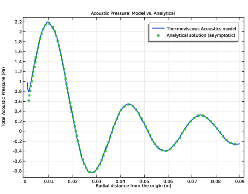
In the associated text field, type Total Acoustic Pressure (Pa).
Line Graph 1
1
Right-click Total Acoustic Pressure and choose Line Graph.
2
In the Settings window for Line Graph, locate the x-Axis Data section.
3
From the Parameter list, choose Expression.
4
In the Expression text field, type R0.
5
Click to expand the Coloring and Style section. In the Width text field, type 2.
6
Click to expand the Legends section. Select the Show legends check box.
7
From the Legends list, choose Manual.
8
Line Graph 2
1
Right-click Line Graph 1 and choose Duplicate.
2
In the Settings window for Line Graph, locate the y-Axis Data section.
3
In the Expression text field, type p_an.
4
Locate the Coloring and Style section. Find the Line markers subsection. From the Marker list, choose Point.
5
Find the Line style subsection. From the Line list, choose None.
6
In the Width text field, type 1.
7
Find the Line markers subsection. In the Number text field, type 100.
8
Locate the Legends section. In the table, enter the following settings:
9
In the Total Acoustic Pressure toolbar, click  Plot.
The figure should look like the one in Figure 4.