|
|
|
|
1
|
|
2
|
In the Select Physics tree, select Acoustics>Pressure Acoustics>Pressure Acoustics, Frequency Domain (acpr).
|
|
3
|
Click Add.
|
|
4
|
Click
|
|
5
|
|
6
|
Click
|
|
1
|
|
2
|
|
1
|
|
2
|
|
3
|
Click Browse.
|
|
4
|
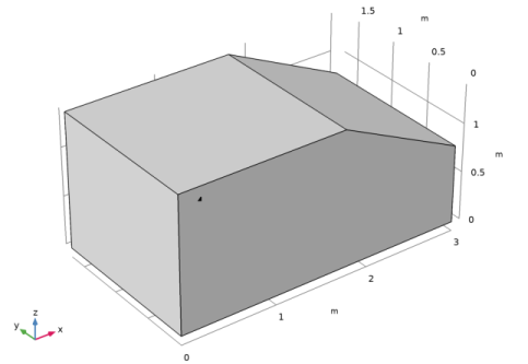
Browse to the model’s Application Libraries folder and double-click the file test_bench_car_interior.mphbin.
|
|
5
|
Click Import.
|
|
1
|
|
2
|
|
3
|
|
4
|
|
1
|
|
2
|
|
3
|
|
4
|
|
5
|
|
1
|
|
2
|
|
3
|
|
1
|
In the Model Builder window, under Component 1 (comp1) right-click Materials and choose Blank Material.
|
|
3
|
|
1
|
In the Model Builder window, under Component 1 (comp1) click Pressure Acoustics, Frequency Domain (acpr).
|
|
2
|
In the Settings window for Pressure Acoustics, Frequency Domain, click to expand the Discretization section.
|
|
3
|
|
1
|
|
3
|
|
4
|
|
1
|
|
2
|
|
1
|
|
2
|
|
3
|
Click the Custom button.
|
|
4
|
|
5
|
|
1
|
|
2
|
|
3
|
|
4
|
|
5
|
|
1
|
|
2
|
|
3
|
In the Model Builder window, expand the Study 1 - L/5 - Direct Solver>Solver Configurations>Solution 1 (sol1)>Stationary Solver 1 node, then click Suggested Direct Solver (acpr).
|
|
4
|
|
5
|
|
6
|
|
1
|
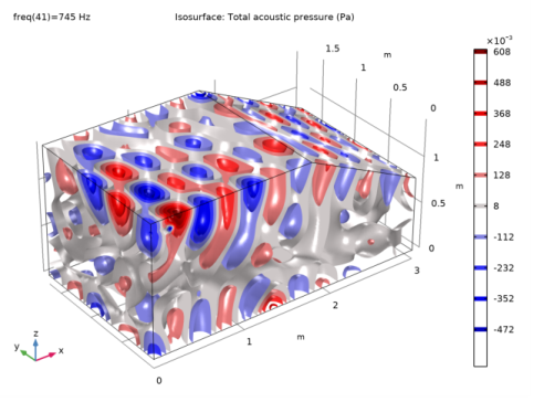
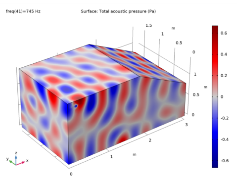
In the Model Builder window, under Results, Ctrl-click to select Acoustic Pressure (acpr), Sound Pressure Level (acpr), and Acoustic Pressure, Isosurfaces (acpr).
|
|
2
|
Right-click and choose Group.
|
|
1
|
|
2
|
|
3
|
|
4
|
|
1
|
|
2
|
|
4
|
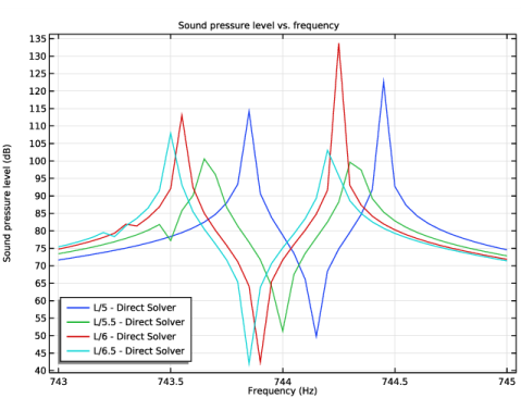
In the Settings window for Point Graph, click Replace Expression in the upper-right corner of the y-Axis Data section. From the menu, choose Component 1 (comp1)>Pressure Acoustics, Frequency Domain>Pressure and sound pressure level>acpr.Lp_t - Total sound pressure level - dB.
|
|
5
|
Click Replace Expression in the upper-right corner of the x-Axis Data section. From the menu, choose Component 1 (comp1)>Pressure Acoustics, Frequency Domain>Global>acpr.freq - Frequency - Hz.
|
|
6
|
|
7
|
|
9
|
|
1
|
|
2
|
|
1
|
|
2
|
|
3
|
|
1
|
|
2
|
|
1
|
|
2
|
|
3
|
|
1
|
|
2
|
|
1
|
|
2
|
|
3
|
|
1
|
|
2
|
|
3
|
|
4
|
|
5
|
|
6
|
|
7
|
|
8
|
|
9
|
|
1
|
|
2
|
|
1
|
|
2
|
|
1
|
|
2
|
|
1
|
|
2
|
|
3
|
|
1
|
|
2
|
|
3
|
|
1
|
|
2
|
|
3
|
|
1
|
|
2
|
|
1
|
|
2
|
|
3
|
In the Model Builder window, expand the Study 2 - L/5.5 - Direct Solver>Solver Configurations>Solution 2 (sol2)>Stationary Solver 1 node, then click Suggested Direct Solver (acpr).
|
|
4
|
|
5
|
|
6
|
|
1
|
In the Model Builder window, under Results, Ctrl-click to select Acoustic Pressure (acpr) 1, Sound Pressure Level (acpr) 1, and Acoustic Pressure, Isosurfaces (acpr) 1.
|
|
2
|
Right-click and choose Group.
|
|
1
|
|
2
|
|
1
|
|
2
|
|
3
|
In the Model Builder window, expand the Study 3 - L/6 - Direct Solver>Solver Configurations>Solution 3 (sol3)>Stationary Solver 1 node, then click Suggested Direct Solver (acpr).
|
|
4
|
|
5
|
|
6
|
|
1
|
In the Model Builder window, under Results, Ctrl-click to select Acoustic Pressure (acpr) 2, Sound Pressure Level (acpr) 2, and Acoustic Pressure, Isosurfaces (acpr) 2.
|
|
2
|
Right-click and choose Group.
|
|
1
|
|
2
|
|
1
|
|
2
|
|
3
|
In the Model Builder window, expand the Study 4 - L/6.5 - Direct Solver>Solver Configurations>Solution 4 (sol4)>Stationary Solver 1 node, then click Suggested Direct Solver (acpr).
|
|
4
|
|
5
|
|
6
|
|
1
|
In the Model Builder window, under Results, Ctrl-click to select Acoustic Pressure (acpr) 3, Sound Pressure Level (acpr) 3, and Acoustic Pressure, Isosurfaces (acpr) 3.
|
|
2
|
Right-click and choose Group.
|
|
1
|
In the Model Builder window, under Results>1D Plot Group 4 right-click Point Graph 1 and choose Duplicate.
|
|
2
|
|
3
|
|
4
|
Locate the Legends section. In the table, enter the following settings:
|
|
1
|
|
2
|
|
3
|
|
4
|
Locate the Legends section. In the table, enter the following settings:
|
|
1
|
|
2
|
|
3
|
|
4
|
Locate the Legends section. In the table, enter the following settings:
|
|
5
|
|
1
|
|
2
|
|
3
|
|
4
|
|
5
|
In the associated text field, type Sound pressure level (dB).
|
|
6
|
|
7
|