PDF

Nonlinear Acoustics — Modeling of the 1D Westervelt Equation
Introduction
Although linear acoustics does an outstanding job of explaining most acoustical phenomena, there are an increasing number of applications that require abandoning the small-signal assumption and applying the wave equation for finite-amplitude sound or nonlinear acoustics. For example, the effects of finite amplitude propagation can be seen in almost every medical use of ultrasound. The use of high intensity ultrasound to induce tissue heating for cancer therapy or bleeding control, and the use of shock waves in extracorporeal and endoscopic lithotripsy of kidney stones and gallstones provide additional examples. Even in the field of diagnostic ultrasound, nonlinear acoustics is of interest because the higher harmonics emerged during wave propagation can be exploited to produce a better image quality.
The nonlinear phenomenon of wave distortion is both a local effect and a cumulative effect due to variation of propagation speed over the waveform, which causes distortion that accumulates with propagation distance. The local effect is usually small compared to cumulative distortion and can be neglected once the propagation distance becomes much greater than a wavelength; see Ref. 1. Therefore, a transient analysis is necessary to model the cumulative distortion along with the wave propagation.
This example shows how to model nonlinear propagation of finite-amplitude acoustic waves in fluids using the Pressure Acoustics, Transient physics interface of the Acoustics Module. The nonlinear effects are taken into account by adding the Nonlinear Acoustics (Westervelt) domain feature. Thus the linear wave equation transforms into the Westervelt equation which is an approximation of the full 2nd-order wave equation when cumulative nonlinear effects dominate local nonlinear effects; see Ref. 1. The current model simulates a finite-amplitude wave propagating in 1D along an interval greater than the shock formation distance. The computed numerical solution is compared to an analytical solution before and after shock formation.
Model Definition
The full Westervelt equation reads
(1)
where p is the total acoustic pressure, ρ0 and c0 are the density and the speed of sound, β = 1 + B/2A is the coefficient of nonlinearity, and δ is the sound diffusivity (see Ref. 2). This is the equation solved when the Nonlinear Acoustics (Westervelt) domain feature is added and the General dissipation is selected as Fluid model is selected on the main Transient Pressure Acoustics Model node.
For a piston vibrating in a 1D tube with the velocity u(t) = u0sinωt, the so-called shock formation distance is
,
There are two classical analytical solutions to Equation 1 available in this case (see Ref. 1). Both of them have the form of a series
(2),
where σ x/xsh is the dimensionless spatial coordinate and p0 = ρ0c0u0 is the source pressure amplitude.
The first one is known as the Fubini solution and is valid for the distances up to xsh (σ ≤ 1). The harmonic amplitudes Bn are defined as
,
with Jn being the Bessel function of the first kind of order n. The second one is known as the Fay solution and it is applied for σ ≥ 3.5. The harmonic amplitudes are
with Γ = 2βu0/ωδ is the Goldberg number, which is a measure of the strength of nonlinearity relative to that of dissipation (see Ref. 1). A solution provided by Blackstock exists in the transition region for 1 ≤ σ ≤ 3.5, but this solution is not considered here.
Table 1 shows the material properties of water and some critical parameters used in the simulation. Given those numbers, the shock formation distance for the current model is about 0.1 m. The simulation domain is the interval 0 ≤ x ≤ 4.5xsh, as shown in Figure 1. A sinusoidal pressure source of amplitude p0 is applied at x = 0, and the Plane Wave Radiation boundary condition is applied at x = 4.5xsh to model the propagation of the wave without reflections. The diffusivity of sound present in the model is due to viscosity and is defined as δ = 4μ/3ρ0. It corresponds to the acoustic attenuation α = 8.1·10-5 Np/m.
ρ0
Density at 20oC and 1 atm
c0
μ0
1.0016·10-3 Pa·s
Viscosity at 20oC and 1 atm
β
f0
p0
N0
Figure 1: 1D geometry of the model with the source located at x = 0.
Results and Discussion
The increasing distortion of the waveform when the wave travels away from the acoustic source is illustrated in Figure 2. The nonlinear effects are apparent by comparing the solution with the linear analytical solution. Initially, the waveform distortion is caused by the dependence of propagation speed on the pressure or particle velocity. The peaks of the wave travel faster than the troughs, and the waveform gradually turns into a sawtooth-like shape clearly seen near the right end of the interval. After the shock formation (the red vertical line in Figure 2) the sound dissipation grows. This is due to the intrinsic frequency dependency of the attenuation. It is proportional to the frequency squared.
The distortion of the waveform results in the generation of higher harmonic components. The further the wave travels, the more energy is transferred to the higher harmonic components from the fundamental frequency of the harmonic source signal. This effect is demonstrated in the plots of Figure 3 through Figure 5. The plots compare the model solution (blue lines) with the analytical solutions (green line) for both waveform and frequency spectrum at x = 0.5xsh, xsh, and 3.5xsh. The Fourier transforms used to determine the spectrum are applied for the time interval Δt = 5T0 after the wave arrives at those locations.
At x = 0.5xsh in Figure 3, the 2nd and the 3rd harmonic components start to show up; at x = xsh in Figure 4, more than ten harmonics appear in the frequency spectrum. Their contribution grows with the distance as seen in Figure 5 at x = 3.5xsh. These results clearly show how the wave deforms when it travels away from the source and how the acoustic energy is pumped into higher harmonics from the fundamental frequency.
Note: The Fubini solution is a solution to Equation 1 with no dissipation (δ = 0). Therefore, the difference in amplitudes of the numerical and the analytical solution grows as x comes closer to xsh (compare plots in Figure 3 and Figure 4).
Figure 2: Comparison of the nonlinear numerical solution (blue) with the linear analytical solution (green): the full propagation domain in the top plot and the area around the shock formation distance in the bottom plot. The red vertical line indicates the shock formation distance.
Figure 3: Comparison of model solution (blue) with Fubini nonlinear analytical solution (green) at x = 0.5xsh. The top plot shows the pressure profiles and the bottom plot shows the frequency spectra.
Figure 4: Comparison of model solution (blue) with Fubini nonlinear analytical solution (green) at x = xsh. The top plot shows the pressure profiles and the bottom plot shows the frequency spectra.
Figure 5: Comparison of model solution (blue) with Fay nonlinear analytical solution (green) at x = 3.5xsh. The top plot shows the pressure profiles and the bottom plot shows the frequency spectra.
Notes About the COMSOL Implementation
Mesh and finite element discretization
The mesh is required to resolves the frequency content of the signal. That means resolving higher harmonics along the wave propagation direction. The specified number of harmonics to resolve N0, should therefore contribute to the mesh element size. To accurately resolve the acoustic pressure, use at least second-order (quadratic) elements. Then the mesh element size is defined as dx = c0/(6N0f0).
Time Stepping
The time stepping depends on the maximum frequency to resolve. It is specified in Transient Solver Settings section at the top physics level. In the model it is selected to resolve the desired number of harmonics as fmax = N0f0. The Generalized alpha time stepping method generated as the default transient solver will automatically use an appropriate time step to resolve up to fmax.
Note that when the Nonlinear Acrostics (Westervelt) feature is used the default solver should be regenerated if, for example, a linear model was solved previously. This is to ensure that a proper solve is set up. The addition of the nonlinear feature will trigger the Automatic (Newton) method for solving the boundary value problem.
Shock-capturing stabilization
Since the model discusses a subject of nonlinear wave propagation beyond the shock-formation distance, a special treatment is required to resolve the discontinuities of the shock. The Nonlinear Acoustics (Westervelt) feature contains a built-in Shock-Capturing Stabilization technique available when Stabilization is enabled in the Show view. The stabilization is turned off per default as it requires manual tuning.
Whenever the Enable q-Laplacian relaxation is enabled, an extra nonlinear term
is added to the sound diffusivity, δ. This nonlinear term introduces additional dissipation that is maximal where the acoustic pressure endures discontinuities, that is, at shocks. The parameters κ and q must be tuned so as not to introduce too much or too little dissipation. The choice depends on the material properties and the frequency of the input signal. In this model, κ = 0.01 and q = 1.35. This simple 1D model can be used to tune the stabilization parameters (for other materials and frequencies) for higher dimension models as it is relatively fast to solve.
References
1. M.F. Hamilton and D.T. Blackstock, eds., Nonlinear Acoustics, Academic Press, San Diego, CA, 1998.
2. D.T. Blackstock, Fundamentals of Physical Acoustics, John Wiley & Sons, 2000.
Application Library path: Acoustics_Module/Nonlinear_Acoustics/nonlinear_acoustics_westervelt_1d
Modeling Instructions
From the File menu, choose New.
New
In the New window, click  Model Wizard.
Model Wizard
1
In the Model Wizard window, click  1D.
2
In the Select Physics tree, select Acoustics>Pressure Acoustics>Pressure Acoustics, Transient (actd).
3
Click Add.
4
Click  Study.
5
In the Select Study tree, select General Studies>Time Dependent.
6
Global Definitions
Load the parameters used in the model from a file. Some of the parameters are presented in Table 1.
Parameters 1
1
In the Model Builder window, under Global Definitions click Parameters 1.
2
In the Settings window for Parameters, locate the Parameters section.
3
Click  Load from File.
4
Now, define the amplitudes Bn used in the Fubini and Fay analytical solutions to Equation 1.
Analytic 1 (an1)
1
In the Home toolbar, click  Functions and choose Global>Analytic.
2
In the Settings window for Analytic, type Pn_fubini in the Function name text field.
3
Locate the Definition section. In the Expression text field, type 1/n*besselj(n, n*sigma)*sin(n*omega0*(t - sigma*x_sh/c0)).
4
In the Arguments text field, type sigma, t, n.
5
Locate the Units section. In the Arguments text field, type 1, s, 1.
6
In the Function text field, type 1.
Analytic 2 (an2)
1
In the Home toolbar, click  Functions and choose Global>Analytic.
2
In the Settings window for Analytic, type Pn_fay in the Function name text field.
3
Locate the Definition section. In the Expression text field, type 1/sinh(n*(sigma + 1)/Gamma)*sin(n*omega0*(t - sigma*x_sh/c0)).
4
In the Arguments text field, type sigma, t, n.
5
Locate the Units section. In the Arguments text field, type 1, s, 1.
6
In the Function text field, type 1.
Define variables for the linear and nonlinear analytical solutions to the problem. Use the sum() operator with 100 terms to approximate the expression given in Equation 2.
Definitions
Variables 1
1
In the Model Builder window, under Component 1 (comp1) right-click Definitions and choose Variables.
2
In the Settings window for Variables, locate the Variables section.
3
Geometry 1
Interval 1 (i1)
1
In the Model Builder window, under Component 1 (comp1) right-click Geometry 1 and choose Interval.
2
In the Settings window for Interval, locate the Interval section.
3
4
Click  Build All Objects.
The geometry should look like the one presented in Figure 1.
Pressure Acoustics, Transient (actd)
1
In the Model Builder window, under Component 1 (comp1) click Pressure Acoustics, Transient (actd).
2
In the Settings window for Pressure Acoustics, Transient, locate the Typical Wave Speed for Perfectly Matched Layers section.
3
In the cref text field, type c0.
4
Locate the Transient Solver Settings section. In the Maximum frequency to resolve field enter N0*f0. It will give the maximal time step for the Transient Solver required to resolve up to N0-harmonics.
Transient Pressure Acoustics Model 1
1
In the Model Builder window, under Component 1 (comp1)>Pressure Acoustics, Transient (actd) click Transient Pressure Acoustics Model 1.
2
In the Settings window for Transient Pressure Acoustics Model, locate the Transient Pressure Acoustics Model section.
3
From the Fluid model list, choose General dissipation.
4
From the c list, choose User defined. In the associated text field, type c0.
5
From the ρ list, choose User defined. In the associated text field, type rho0.
6
From the δ list, choose User defined. In the associated text field, type d_diff.
Nonlinear Acoustics (Westervelt) Contributions 1
1
In the Physics toolbar, click  Domains and choose Nonlinear Acoustics (Westervelt) Contributions.
2
3
In the Settings window for Nonlinear Acoustics (Westervelt) Contributions, locate the Nonlinear Acoustics (Westervelt) Contributions section.
4
From the Specify list, choose Coefficient of nonlinearity.
5
In the β text field, type beta.
Since the computational domain is larger than the shock formation distance, shocks form as the wave passes xsh. Therefore it is required to enable the shock-capturing stabilization to resolve the shocks.
6
Click the  Show More Options button in the Model Builder toolbar.
7
In the Show More Options dialog box, in the tree, select the check box for the node Physics>Stabilization.
8
9
In the Model Builder window, click Nonlinear Acoustics (Westervelt) Contributions 1.
10
In the Settings window for Nonlinear Acoustics (Westervelt) Contributions, click to expand the Shock-Capturing Stabilization section.
11
Select the Enable q-Laplacian relaxation check box.
12
In the q text field, type 1.35.
13
In the κ text field, type 0.01.
Pressure 1
1
In the Physics toolbar, click  Boundaries and choose Pressure.
2
3
In the Settings window for Pressure, locate the Pressure section.
4
In the p0 text field, type P0*sin(omega0*t).
Plane Wave Radiation 1
1
In the Physics toolbar, click  Boundaries and choose Plane Wave Radiation.
2
Mesh 1
1
In the Model Builder window, under Component 1 (comp1) click Mesh 1.
2
In the Settings window for Mesh, locate the Mesh Settings section.
3
From the Sequence type list, choose User-controlled mesh.
Size
1
In the Model Builder window, under Component 1 (comp1)>Mesh 1 click Size.
2
In the Settings window for Size, locate the Element Size section.
3
Click the Custom button.
4
Locate the Element Size Parameters section. In the Maximum element size text field, type DX.
5
Click  Build All.
Study 1
Step 1: Time Dependent
1
In the Model Builder window, under Study 1 click Step 1: Time Dependent.
2
In the Settings window for Time Dependent, locate the Study Settings section.
3
In the Output times text field, type range(0,T0/50,Nt*T0).
4
In the Home toolbar, click  Compute.
Results
Acoustic Pressure (actd)
1
In the Settings window for 1D Plot Group, locate the Data section.
2
From the Time selection list, choose Last.
3
Locate the Plot Settings section. Select the x-axis label check box.
4
Select the y-axis label check box.
5
6
Click to expand the Title section. From the Title type list, choose Manual.
7
In the Title text area, type Total acoustic pressure field (Pa).
Line Graph 1
1
In the Model Builder window, expand the Acoustic Pressure (actd) node, then click Line Graph 1.
2
In the Settings window for Line Graph, click to expand the Legends section.
3
Select the Show legends check box.
4
From the Legends list, choose Manual.
5
Line Graph 2
1
In the Model Builder window, right-click Acoustic Pressure (actd) and choose Line Graph.
2
3
In the Settings window for Line Graph, locate the y-Axis Data section.
4
In the Expression text field, type p_linear.
5
Locate the Legends section. Select the Show legends check box.
6
From the Legends list, choose Manual.
7
8
Locate the x-Axis Data section. From the Parameter list, choose Expression.
9
In the Expression text field, type x.
Line Graph 3
1
Right-click Acoustic Pressure (actd) and choose Line Graph.
2
3
In the Settings window for Line Graph, locate the x-Axis Data section.
4
From the Parameter list, choose Expression.
5
In the Expression text field, type x_sh.
6
Click to expand the Coloring and Style section. In the Width text field, type 2.
7
Locate the Legends section. Select the Show legends check box.
8
From the Legends list, choose Manual.
9
10
In the Acoustic Pressure (actd) toolbar, click  Plot.
The plot should look like the top plot in Figure 2.
You can examine the plot in greater detail by zooming around parts of the plot using the Zoom Box tool as shown in the bottom plot in Figure 2.
Create Cut Points to compare the numerical solution with the analytical ones at x = 0.5xsh, xsh, and 3.5xsh.
Cut Point - 0.5 Shock
1
In the Results toolbar, click  More Datasets and choose Cut Point 1D.
2
In the Settings window for Cut Point 1D, locate the Point Data section.
3
In the X text field, type 0.5*x_sh.
4
In the Label text field, type Cut Point - 0.5 Shock.
Cut Point - 1 Shock
1
In the Results toolbar, click  More Datasets and choose Cut Point 1D.
2
In the Settings window for Cut Point 1D, locate the Point Data section.
3
In the X text field, type x_sh.
4
In the Label text field, type Cut Point - 1 Shock.
Cut Point - 3.5 Shock
1
In the Results toolbar, click  More Datasets and choose Cut Point 1D.
2
In the Settings window for Cut Point 1D, locate the Point Data section.
3
In the X text field, type 3.5*x_sh.
4
In the Label text field, type Cut Point - 3.5 Shock.
Plot the numerical and the analytical solutions at Cut Points.
Acoustic Pressure at sigma = 0.5
1
In the Results toolbar, click  1D Plot Group.
2
In the Settings window for 1D Plot Group, type Acoustic Pressure at sigma = 0.5 in the Label text field.
3
Locate the Data section. From the Dataset list, choose Cut Point - 0.5 Shock.
4
From the Time selection list, choose Interpolated.
5
In the Times (s) text field, type range((Nt - 5)*T0, T0/50, Nt*T0).
6
Locate the Plot Settings section. Select the y-axis label check box.
7
8
Locate the Title section. From the Title type list, choose Manual.
9
In the Title text area, type Comparison to analytical solution at sigma = 0.5.
Point Graph 1
1
Right-click Acoustic Pressure at sigma = 0.5 and choose Point Graph.
2
In the Settings window for Point Graph, click to expand the Legends section.
3
Select the Show legends check box.
4
From the Legends list, choose Manual.
5
Point Graph 2
1
In the Model Builder window, right-click Acoustic Pressure at sigma = 0.5 and choose Point Graph.
2
In the Settings window for Point Graph, locate the y-Axis Data section.
3
In the Expression text field, type p_fubini.
4
Locate the Legends section. Select the Show legends check box.
5
From the Legends list, choose Manual.
6
7
In the Acoustic Pressure at sigma = 0.5 toolbar, click  Plot.
The plot should look like the top plot in Figure 3.
Acoustic Pressure at sigma = 1
1
In the Home toolbar, click  Add Plot Group and choose 1D Plot Group.
2
In the Settings window for 1D Plot Group, type Acoustic Pressure at sigma = 1 in the Label text field.
3
Locate the Data section. From the Dataset list, choose Cut Point - 1 Shock.
4
From the Time selection list, choose Interpolated.
5
In the Times (s) text field, type range((Nt - 5)*T0, T0/50, Nt*T0).
6
Locate the Plot Settings section. Select the y-axis label check box.
7
8
Locate the Title section. From the Title type list, choose Manual.
9
In the Title text area, type Comparison to analytical solution at sigma = 1.
Point Graph 1
1
Right-click Acoustic Pressure at sigma = 1 and choose Point Graph.
2
In the Settings window for Point Graph, locate the Legends section.
3
Select the Show legends check box.
4
From the Legends list, choose Manual.
5
Point Graph 2
1
In the Model Builder window, right-click Acoustic Pressure at sigma = 1 and choose Point Graph.
2
In the Settings window for Point Graph, locate the y-Axis Data section.
3
In the Expression text field, type p_fubini.
4
Locate the Legends section. Select the Show legends check box.
5
From the Legends list, choose Manual.
6
7
In the Acoustic Pressure at sigma = 1 toolbar, click  Plot.
The plot should look like the top plot in Figure 4.
Acoustic Pressure at sigma = 3.5
1
In the Home toolbar, click  Add Plot Group and choose 1D Plot Group.
2
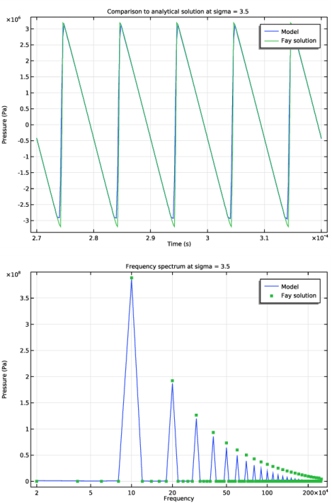
In the Settings window for 1D Plot Group, type Acoustic Pressure at sigma = 3.5 in the Label text field.
3
Locate the Data section. From the Dataset list, choose Cut Point - 3.5 Shock.
4
From the Time selection list, choose Interpolated.
5
In the Times (s) text field, type range((Nt - 5)*T0, T0/50, Nt*T0).
6
Locate the Plot Settings section. Select the y-axis label check box.
7
8
Locate the Title section. From the Title type list, choose Manual.
9
In the Title text area, type Comparison to analytical solution at sigma = 3.5.
Point Graph 1
1
Right-click Acoustic Pressure at sigma = 3.5 and choose Point Graph.
2
In the Settings window for Point Graph, locate the Legends section.
3
Select the Show legends check box.
4
From the Legends list, choose Manual.
5
Point Graph 2
1
In the Model Builder window, right-click Acoustic Pressure at sigma = 3.5 and choose Point Graph.
2
In the Settings window for Point Graph, locate the y-Axis Data section.
3
In the Expression text field, type p_fay.
4
Locate the Legends section. Select the Show legends check box.
5
From the Legends list, choose Manual.
6
7
In the Acoustic Pressure at sigma = 3.5 toolbar, click  Plot.
The plot should look like the top plot in Figure 5.
Acoustic Pressure Spectrum at sigma = 0.5
1
In the Model Builder window, right-click Acoustic Pressure at sigma = 0.5 and choose Duplicate.
2
In the Settings window for 1D Plot Group, type Acoustic Pressure Spectrum at sigma = 0.5 in the Label text field.
3
Locate the Title section. In the Title text area, type Frequency spectrum at sigma = 0.5.
4
Click the  x-Axis Log Scale button in the Graphics toolbar.
Point Graph 1
1
In the Model Builder window, expand the Acoustic Pressure Spectrum at sigma = 0.5 node, then click Point Graph 1.
2
In the Settings window for Point Graph, locate the x-Axis Data section.
3
From the Parameter list, choose Frequency spectrum.
Point Graph 2
1
In the Model Builder window, click Point Graph 2.
2
In the Settings window for Point Graph, locate the x-Axis Data section.
3
From the Parameter list, choose Frequency spectrum.
4
Click to expand the Coloring and Style section. Find the Line style subsection. From the Line list, choose None.
5
Find the Line markers subsection. From the Marker list, choose Point.
6
From the Positioning list, choose In data points.
7
In the Acoustic Pressure Spectrum at sigma = 0.5 toolbar, click  Plot.
The plot should look like the bottom plot in Figure 3.
Acoustic Pressure Spectrum at sigma = 1
1
In the Model Builder window, right-click Acoustic Pressure at sigma = 1 and choose Duplicate.
2
In the Settings window for 1D Plot Group, type Acoustic Pressure Spectrum at sigma = 1 in the Label text field.
3
Click to expand the Title section. In the Title text area, type Frequency spectrum at sigma = 1.
4
Click the  x-Axis Log Scale button in the Graphics toolbar.
Point Graph 1
1
In the Model Builder window, expand the Acoustic Pressure Spectrum at sigma = 1 node, then click Point Graph 1.
2
In the Settings window for Point Graph, locate the x-Axis Data section.
3
From the Parameter list, choose Frequency spectrum.
Point Graph 2
1
In the Model Builder window, click Point Graph 2.
2
In the Settings window for Point Graph, locate the x-Axis Data section.
3
From the Parameter list, choose Frequency spectrum.
4
Locate the Coloring and Style section. Find the Line style subsection. From the Line list, choose None.
5
Find the Line markers subsection. From the Marker list, choose Point.
6
From the Positioning list, choose In data points.
7
In the Acoustic Pressure Spectrum at sigma = 1 toolbar, click  Plot.
The plot should look like the bottom plot in Figure 4.
Acoustic Pressure Spectrum at sigma = 3.5
1
In the Model Builder window, right-click Acoustic Pressure at sigma = 3.5 and choose Duplicate.
2
In the Settings window for 1D Plot Group, type Acoustic Pressure Spectrum at sigma = 3.5 in the Label text field.
3
Locate the Title section. In the Title text area, type Frequency spectrum at sigma = 3.5.
4
Click the  x-Axis Log Scale button in the Graphics toolbar.
Point Graph 1
1
In the Model Builder window, expand the Acoustic Pressure Spectrum at sigma = 3.5 node, then click Point Graph 1.
2
In the Settings window for Point Graph, locate the x-Axis Data section.
3
From the Parameter list, choose Frequency spectrum.
Point Graph 2
1
In the Model Builder window, click Point Graph 2.
2
In the Settings window for Point Graph, locate the x-Axis Data section.
3
From the Parameter list, choose Frequency spectrum.
4
Locate the Coloring and Style section. Find the Line style subsection. From the Line list, choose None.
5
Find the Line markers subsection. From the Marker list, choose Point.
6
From the Positioning list, choose In data points.
7
In the Acoustic Pressure Spectrum at sigma = 3.5 toolbar, click  Plot.
The plot should look like the bottom plot in Figure 5.