PDF

Hollow Cylinder
Introduction
Fluid acoustics coupled to structural objects (vibroacoustics), such as membranes or plates, represents an important application area in many engineering fields. Some examples are loudspeakers, acoustic sensors, nondestructive impedance testing, and medical ultrasound diagnostics of the human body. Through the use of the Acoustic - Solid Interaction, Frequenccy Domain multiphysics interface, this model demonstrates how fluid acoustics can be easily coupled to structures.
Model Definition
This model provides a general demonstration of an acoustic fluid phenomenon in 3D coupled to a solid object. In this study, the solid object is a capped, hollow aluminum cylinder filled with and immersed in water. The acoustic waves created by a source inside the cylinder impact the cylinder walls.
Figure 1: A hollow aluminum cylinder is immersed in water. The white line inside the cylinder indicates the line source, and the tiny sphere next to the line shows the position of the point source. The simulation domain is bounded by a large sphere.
Figure 1 illustrates the aluminum cylinder immersed in water. The cylinder is 2 cm in height and has an outer diameter of 1 cm. The thickness of its walls is 0.5 mm.
The water-filled acoustic domain outside the cylinder is truncated to a sphere with a reasonably large diameter. In two different versions of the model, the system is driven either by a line source coinciding with the axis of the cylinder and located entirely within the cylinder or by a point source in the interior of the cylinder. The frequency studied is 60 kHz, that is, in the ultrasound region. The fluid and solid domains are coupled using the built-in Acoustic-Structure Boundary multiphysics coupling. The coupling ensures a fully two-way coupled analysis of the problem.
Domain and Boundary Conditions
Water Domain
For harmonic sound waves, in the frequency domain, the model solves the Helmholtz equation defined in the Pressure Acoustics, Frequency Domain interface.
Solid Domain
You calculate the harmonic stresses and strains inside the solid cylinder walls using the same equation formulation as a frequency response analysis in the 3D Solid Mechanics interface. The material data comes from the built-in database for Aluminum 3003-H18.
Outer Perimeter
On the outer spherical perimeter of the water domain (Figure 1), use the predefined Spherical Wave Radiation condition. This boundary condition allows a spherical wave to travel out of the system, giving only slight reflections for the non-spherical components of the wave. For mathematical details on the radiation boundary condition, see the Acoustics Module User’s Guide.
Cylinder-Water Interface
The model uses the Acoustic-Solid Interaction, Frequency Domain multiphysics interface, in which the Acoustic-Structure Boundary multiphysics coupling condition automatically apply to all acoustic-structure boundaries. The condition ensures that the acoustic pressure is added as a load on the solid and that the solid normal acceleration is added as a source on the acoustic domain.
edge and point settings
In the two cases considered, the sound waves are generated by either a point monopole source or a line source. A line source along the z-axis defines the following right-hand-side source term to the Helmholtz equation:
Here Prms is the free space reference rms power per unit length of a line source of length Ledge placed in a homogeneous medium extending to infinity. Furthermore, δ(2)(r) is the Dirac delta function in two dimensions, r denoting the projection of the position vector onto the xy-plane.
A monopole point source of rms power Prms  located at the point R = R0 in an infinite homogeneous space defined the following source term
where δ(3)(R) is the Dirac delta function in three dimensions. Any type of confinement results in higher power usage.
Results
Figure 2 shows the resulting deformations and local sound pressure level from a computation with a line source.
Figure 2: Sound-pressure level plot (dB) of the acoustic waves in the coupled problem, using a line source inside the cylinder. The surface of the cylinder shows its deformation (mm).
In Figure 3, you see the solution from an off-centered point. Note that the deformation color scale is different, implying that this source gives deformations that at least locally are greater than those from the line source.
Figure 3: Sound-pressure level (dB) and structural deformations (mm) with a point source inside the cylinder. Some of the surfaces are hidden to reveal the pressure distribution inside the cylinder.
Application Library path: Acoustics_Module/Vibrations_and_FSI/hollow_cylinder
Modeling Instructions
From the File menu, choose New.
New
In the New window, click  Model Wizard.
Model Wizard
1
In the Model Wizard window, click  3D.
2
In the Select Physics tree, select Acoustics>Acoustic-Structure Interaction>Acoustic-Solid Interaction, Frequency Domain.
3
Click Add.
4
Click  Study.
5
In the Select Study tree, select General Studies>Frequency Domain.
6
Global Definitions
Parameters 1
1
In the Model Builder window, under Global Definitions click Parameters 1.
2
In the Settings window for Parameters, locate the Parameters section.
3
Geometry 1
1
In the Model Builder window, under Component 1 (comp1) click Geometry 1.
2
In the Settings window for Geometry, locate the Units section.
3
From the Length unit list, choose mm.
Cylinder 1 (cyl1)
1
In the Geometry toolbar, click  Cylinder.
2
In the Settings window for Cylinder, locate the Size and Shape section.
3
In the Radius text field, type cylr.
4
In the Height text field, type cylh.
5
Locate the Position section. In the z text field, type -cylh/2.
6
Click to expand the Layers section. Select the Layers on bottom check box.
7
Select the Layers on top check box.
8
9
Click  Build All Objects.
10
Click the  Wireframe Rendering button in the Graphics toolbar.
With wireframe rendering, you now see the contours of both cylinders.
Line Segment 1 (ls1)
1
In the Geometry toolbar, click  More Primitives and choose Line Segment.
2
In the Settings window for Line Segment, locate the Starting Point section.
3
From the Specify list, choose Coordinates.
4
Locate the Endpoint section. From the Specify list, choose Coordinates.
5
Locate the Starting Point section. In the y text field, type (cylr-cylth)/3.
6
In the z text field, type -edgeL/2.
7
Locate the Endpoint section. In the y text field, type (cylr-cylth)/3.
8
In the z text field, type edgeL/2.
Point 1 (pt1)
1
In the Geometry toolbar, click  More Primitives and choose Point.
2
In the Settings window for Point, locate the Point section.
3
In the x text field, type (cylr-cylth)/3.
4
In the y text field, type (cylr-cylth)*2/3.
5
In the z text field, type (cylh/2-cylth)/3.
Sphere 1 (sph1)
1
In the Geometry toolbar, click  Sphere.
2
In the Settings window for Sphere, locate the Size section.
3
In the Radius text field, type 1.5*cylh.
4
Click  Build All Objects.
5
Click the  Zoom Extents button in the Graphics toolbar.
The geometry should look like this.
Definitions
Solid
1
In the Definitions toolbar, click  Explicit.
2
In the Settings window for Explicit, type Solid in the Label text field.
3
Water
1
In the Definitions toolbar, click  Explicit.
2
In the Settings window for Explicit, type Water in the Label text field.
3
Line Source
1
In the Definitions toolbar, click  Explicit.
2
In the Settings window for Explicit, type Line Source in the Label text field.
3
Locate the Input Entities section. From the Geometric entity level list, choose Edge.
4
This is the line that will act as a source. The selection should look like this.
Point Source
1
In the Definitions toolbar, click  Explicit.
2
In the Settings window for Explicit, type Point Source in the Label text field.
3
Locate the Input Entities section. From the Geometric entity level list, choose Point.
4
Point 32 lies inside the cylinder and is the only point that is not connected to any edges. The selection should look like this.
Add Material
1
In the Home toolbar, click  Add Material to open the Add Material window.
2
Go to the Add Material window.
3
In the tree, select Built-in>Water, liquid.
4
Click Add to Component in the window toolbar.
5
In the tree, select Built-in>Aluminum 3003-H18.
6
Click Add to Component in the window toolbar.
7
In the Home toolbar, click  Add Material to close the Add Material window.
Materials
Water, liquid (mat1)
1
In the Model Builder window, under Component 1 (comp1)>Materials click Water, liquid (mat1).
2
In the Settings window for Material, locate the Geometric Entity Selection section.
3
From the Selection list, choose Water.
Aluminum 3003-H18 (mat2)
1
In the Model Builder window, click Aluminum 3003-H18 (mat2).
2
In the Settings window for Material, locate the Geometric Entity Selection section.
3
From the Selection list, choose Solid.
Pressure Acoustics, Frequency Domain (acpr)
By default, all domains are using the Pressure Acoustics model, which holds for fluids. Use the Water selection to specify where Pressure Acoustics is applied.
1
In the Model Builder window, under Component 1 (comp1) click Pressure Acoustics, Frequency Domain (acpr).
2
In the Settings window for Pressure Acoustics, Frequency Domain, locate the Domain Selection section.
3
From the Selection list, choose Water.
4
Locate the Sound Pressure Level Settings section. From the Reference pressure for the sound pressure level list, choose Use reference pressure for water.
The water reference pressure is 1 µPa. This does not affect the physics, but only serves as a reference in the definition of the sound pressure level.
Spherical Wave Radiation 1
1
In the Physics toolbar, click  Boundaries and choose Spherical Wave Radiation.
2
These are the boundaries that will have a radiation condition on them. The selection should look like this.
Line Source 1
1
In the Physics toolbar, click  Edges and choose Line Source.
2
In the Settings window for Line Source, locate the Edge Selection section.
3
From the Selection list, choose Line Source.
4
Locate the Line Source section. From the Type list, choose Power.
5
In the Prms text field, type 0.5.
Monopole Point Source 1
1
In the Physics toolbar, click  Points and choose Monopole Point Source.
2
In the Settings window for Monopole Point Source, locate the Point Selection section.
3
From the Selection list, choose Point Source.
4
Locate the Monopole Point Source section. From the Type list, choose Power.
5
In the Prms text field, type 0.5.
You will select either the line source or the point source under the study by enabling Modify physics tree and variables for study step.
Solid Mechanics (solid)
1
In the Model Builder window, under Component 1 (comp1) click Solid Mechanics (solid).
2
In the Settings window for Solid Mechanics, locate the Domain Selection section.
3
From the Selection list, choose Solid.
Multiphysics
Now is a good time to inspect the Multiphysics node. Notice that the Acoustic-Structure Boundary feature is automatically added to all boundaries, but only applied to the boundaries that have water on one side and the solid on the other.
Mesh 1
1
In the Model Builder window, under Component 1 (comp1) click Mesh 1.
2
In the Settings window for Mesh, locate the Mesh Settings section.
3
From the Sequence type list, choose User-controlled mesh.
Size
1
In the Model Builder window, under Component 1 (comp1)>Mesh 1 click Size.
2
In the Settings window for Size, locate the Element Size section.
3
Click the Custom button.
4
Locate the Element Size Parameters section. In the Maximum element size text field, type lam0/5.
This value, combined with the default choice of second-order elements, makes sure that the rule-of-thumb minimum of 10-12 degrees of freedom per wavelength for the solution to be reliable is satisfied.
5
In the Minimum element size text field, type lam0/10.
6
Click  Build Selected.
Free Quad 1
1
In the Mesh toolbar, click  Boundary and choose Free Quad.
2
The model uses some free quad mesh to control what will be the sweep direction in the solid.
Size 1
1
Right-click Free Quad 1 and choose Size.
2
In the Settings window for Size, locate the Element Size section.
3
Click the Custom button.
4
Locate the Element Size Parameters section. Select the Maximum element size check box.
5
6
Select the Minimum element size check box.
7
8
Click  Build Selected.
Swept 1
1
In the Mesh toolbar, click  Swept.
2
In the Settings window for Swept, locate the Domain Selection section.
3
From the Geometric entity level list, choose Domain.
4
From the Selection list, choose Solid.
Distribution 1
1
Right-click Swept 1 and choose Distribution.
With the sweep operation, the 2D mesh previously created will be sweep through the domains. In general it is recommended to have at least two quadratic elements through the thickness.
2
In the Settings window for Distribution, locate the Distribution section.
3
In the Number of elements text field, type 2.
4
Click  Build All.
Study 1 - Line Source
1
In the Model Builder window, click Study 1.
2
In the Settings window for Study, type Study 1 - Line Source in the Label text field.
Step 1: Frequency Domain
1
In the Model Builder window, under Study 1 - Line Source click Step 1: Frequency Domain.
2
In the Settings window for Frequency Domain, locate the Study Settings section.
3
In the Frequencies text field, type f0.
Now, disable the point source by modifying the physics tree.
4
Locate the Physics and Variables Selection section. Select the Modify model configuration for study step check box.
5
In the Physics and variables selection tree, select Component 1 (comp1)>Pressure Acoustics, Frequency Domain (acpr)>Monopole Point Source 1.
6
Click  Disable.
7
In the Home toolbar, click  Compute.
The default plots include all the surfaces of the model, obscuring the cylinder. A selection added to the dataset will make sure that the plots shows the requested variables on the selection.
Results
Study 1 - Line Source/Solution 1 (sol1)
In the Model Builder window, expand the Results>Datasets node, then click Study 1 - Line Source/Solution 1 (sol1).
Selection
1
In the Results toolbar, click  Attributes and choose Selection.
2
In the Settings window for Selection, locate the Geometric Entity Selection section.
3
From the Geometric entity level list, choose Boundary.
4
The selection should look like this.
Four default plots are created after running this model. In the following steps a additional plots will be added to show the space distribution of the acoustic field.
Slice 1
1
In the Model Builder window, right-click Acoustic Pressure (acpr) and choose Slice.
2
In the Settings window for Slice, locate the Plane Data section.
3
From the Plane list, choose ZX-planes.
4
In the Planes text field, type 1.
5
Click to expand the Inherit Style section. From the Plot list, choose Surface 1.
6
In the Acoustic Pressure (acpr) toolbar, click  Plot.
The plot should look like this.
Slice 1
1
In the Model Builder window, right-click Sound Pressure Level (acpr) and choose Slice.
2
In the Settings window for Slice, locate the Expression section.
3
In the Expression text field, type acpr.Lp_t.
4
Locate the Plane Data section. From the Plane list, choose ZX-planes.
5
In the Planes text field, type 1.
6
Locate the Inherit Style section. From the Plot list, choose Surface 1.
7
In the Sound Pressure Level (acpr) toolbar, click  Plot.
The plot should look like this.
Filter 1
1
In the Model Builder window, expand the Results>Acoustic Pressure, Isosurfaces (acpr) node.
2
Right-click Isosurface 1 and choose Filter.
3
In the Settings window for Filter, locate the Element Selection section.
4
In the Logical expression for inclusion text field, type x>0.
Surface 1
1
In the Model Builder window, right-click Acoustic Pressure, Isosurfaces (acpr) and choose Surface.
2
In the Settings window for Surface, click to expand the Inherit Style section.
3
From the Plot list, choose Isosurface 1.
4
In the Acoustic Pressure, Isosurfaces (acpr) toolbar, click  Plot.
The plot should look like this.
Create a new plot of the deformation and sound pressure level. Then proceed to solving the system again with a monopole point source.
Displacement/SPL - Line Source
1
In the Home toolbar, click  Add Plot Group and choose 3D Plot Group.
2
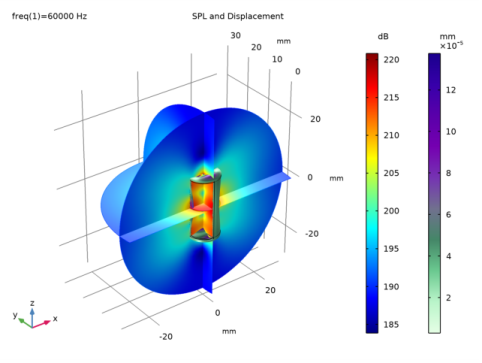
In the Settings window for 3D Plot Group, type Displacement/SPL - Line Source in the Label text field.
3
Click to expand the Title section. From the Title type list, choose Manual.
4
In the Title text area, type SPL and Displacement.
5
Locate the Color Legend section. Select the Show units check box.
Multislice 1
1
In the Displacement/SPL - Line Source toolbar, click  More Plots and choose Multislice.
2
In the Settings window for Multislice, locate the Expression section.
3
In the Expression text field, type acpr.Lp_t.
Add a filter to only show the SPL in the water domain outside of the hollow cylinder.
Filter 1
1
Right-click Multislice 1 and choose Filter.
2
In the Settings window for Filter, locate the Element Selection section.
3
In the Logical expression for inclusion text field, type y>-(cylr-cylth).
Surface 1
1
In the Model Builder window, right-click Displacement/SPL - Line Source and choose Surface.
2
In the Settings window for Surface, locate the Expression section.
3
In the Expression text field, type solid.disp.
4
Locate the Coloring and Style section. From the Color table list, choose AuroraBorealis.
Deformation 1
1
Right-click Surface 1 and choose Deformation.
2
In the Displacement/SPL - Line Source toolbar, click  Plot.
Your plot should now look like Figure 2. The remaining instructions show you how to set up a second study and replace the line source with a point source, while disabling the line source.
Create a group with all plots to facilitate the navigation through the different results.
Acoustic Pressure (acpr), Acoustic Pressure, Isosurfaces (acpr), Displacement/SPL - Line Source, Sound Pressure Level (acpr), Stress (solid)
1
In the Model Builder window, under Results, Ctrl-click to select Acoustic Pressure (acpr), Sound Pressure Level (acpr), Acoustic Pressure, Isosurfaces (acpr), Stress (solid), and Displacement/SPL - Line Source.
2
Plots - Line Source
In the Settings window for Group, type Plots - Line Source in the Label text field.
Add Study
1
In the Home toolbar, click  Add Study to open the Add Study window.
2
Go to the Add Study window.
3
Find the Studies subsection. In the Select Study tree, select General Studies>Frequency Domain.
4
Click Add Study in the window toolbar.
5
In the Home toolbar, click  Add Study to close the Add Study window.
Study 2 - Point Source
1
In the Model Builder window, click Study 2.
2
In the Settings window for Study, type Study 2 - Point Source in the Label text field.
Step 1: Frequency Domain
1
In the Model Builder window, under Study 2 - Point Source click Step 1: Frequency Domain.
2
In the Settings window for Frequency Domain, locate the Study Settings section.
3
In the Frequencies text field, type f0.
4
Locate the Physics and Variables Selection section. Select the Modify model configuration for study step check box.
5
In the Physics and variables selection tree, select Component 1 (comp1)>Pressure Acoustics, Frequency Domain (acpr)>Line Source 1.
6
Click  Disable.
7
In the Home toolbar, click  Compute.
The results for the second study will also include a selection.
Results
Study 2 - Point Source/Solution 2 (sol2)
In the Model Builder window, under Results>Datasets click Study 2 - Point Source/Solution 2 (sol2).
Selection
1
In the Results toolbar, click  Attributes and choose Selection.
2
In the Settings window for Selection, locate the Geometric Entity Selection section.
3
From the Geometric entity level list, choose Boundary.
4
The selection should look like this.
Displacement/SPL - Point Source
1
In the Results toolbar, click  3D Plot Group.
2
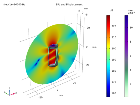
In the Settings window for 3D Plot Group, type Displacement/SPL - Point Source in the Label text field.
3
Locate the Title section. From the Title type list, choose Manual.
4
In the Title text area, type SPL and Displacement.
5
Locate the Color Legend section. Select the Show units check box.
6
Locate the Data section. From the Dataset list, choose Study 2 - Point Source/Solution 2 (sol2).
Slice 1
1
Right-click Displacement/SPL - Point Source and choose Slice.
2
In the Settings window for Slice, locate the Plane Data section.
3
From the Plane list, choose ZX-planes.
4
In the Planes text field, type 1.
5
Locate the Expression section. In the Expression text field, type acpr.Lp_t.
Surface 1
1
In the Model Builder window, right-click Displacement/SPL - Point Source and choose Surface.
2
In the Settings window for Surface, locate the Expression section.
3
In the Expression text field, type solid.disp.
4
Locate the Coloring and Style section. From the Color table list, choose AuroraBorealis.
Deformation 1
1
Right-click Surface 1 and choose Deformation.
2
In the Displacement/SPL - Point Source toolbar, click  Plot.
3
Click the  Zoom Extents button in the Graphics toolbar.
You can see the resulting plot in Figure 3.
Create a group with all plots to facilitate the navigation through the different results.
Acoustic Pressure (acpr) 1, Acoustic Pressure, Isosurfaces (acpr) 1, Displacement/SPL - Point Source, Sound Pressure Level (acpr) 1, Stress (solid) 1
1
In the Model Builder window, under Results, Ctrl-click to select Acoustic Pressure (acpr) 1, Sound Pressure Level (acpr) 1, Acoustic Pressure, Isosurfaces (acpr) 1, Stress (solid) 1, and Displacement/SPL - Point Source.
2
Plots - Point Source
In the Settings window for Group, type Plots - Point Source in the Label text field.