Head and Torso HRTF Computation

This tutorial model shows how to import a 3D scanned geometry of a human head and torso and compute the head related transfer function (HRTF). The scan is imported as a stl file and converted into a COMSOL geometry. The HRTF is computed using the reciprocity principle, locating the source at the ear canal entrance; this approach greatly reduces the computational cost to get a full 3D response. The acoustics are modeled using the Pressure Acoustics, Boundary Element interface of the Acoustics Module. The simulated results are compared to measured data form the actual subject and show good agreement.

The HRTF gives a complete description of the way the head and torso of an individual distorts incident sound fields. The HRTF is an important component of spatial hearing. The HRTF includes both so-called monaural and binaural cues. Binaural cues include the interaural time differenced (ITD) and interaural level differences (ILD), whereas the monaural cues represent a spectral distortion of the sound that is identical for both ears, see Ref. 1. The HRTF is defined as the sound pressure level (SPL) measured at the eardrum (or the ear canal entrance as in this model) relative to the SPL when no head is present.

When virtual sound is used (or acoustic virtual reality) the HRTF is important in order to make the test subject experience a virtual sound scene. The HRTF can be measured, which can be a tedious task, or it can be simulated based on a scan of the individual. This model presents the latter approach on a scanned head geometry provided by the Teaching and Research Area of Medical Acoustics, Institute of Technical Acoustics, RWTH Aachen University, Germany, Ref. 2. The scan is of an actual individual where the facial features have been removed, while all the details of the ear geometry have been retained.

The scanned geometry (stl mesh) and measured data is with courtesy of the Teaching and Research Area of Medical Acoustics, Institute of Technical Acoustics, RWTH Aachen University, Germany. The stl mesh is licensed under the Creative Commons Attribution 4.0 International License and is provided “as is” with all warranties disclaimed, as stated in that license. See Ref. 7 and Ref. 8 for details.

Model Definition

A common approach when simulating the HRTF is to use the reciprocity principle; the source and receiver locations are reverted, Ref. 3. This means that, in the model, the source is located at the entrance of the ear canal and the evaluation is performed along a circle (or on a sphere for the full bubble) with its center in the middle of the head, between the ears. In this way, the HRTF can be deduced for all spatial directions for each frequency with just one simulation. Not using reciprocity requires solving one problem per incidence direction per frequency, which is not practical. Reciprocity is used for similar application in Ref. 4 and Ref. 5.

The acoustic problem is modeled using the boundary element method (BEM) with the Pressure Acoustics, Boundary Element interface. This is especially efficient since the present model represents is a pure radiation problem.

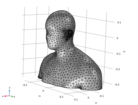
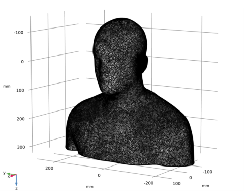
The imported stl mesh is depicted in Figure 1 and the COMSOL geometry generated from the stl mesh is depicted in Figure 2. Notice that the geometry has been moved and rotated (in Figure 2) to align the coordinate axis with the commonly used directions for directivity assessment. The evaluation circle for the HRTF that is use in the model, is represented in Figure 2. The evaluation is performed using a Radiation Pattern plot.

Figure 1: The imported stl mesh. The imported stl mesh is courtesy of the Teaching and Research Area of Medical Acoustics, Institute of Technical Acoustics, RWTH Aachen University, Germany. The stl mesh is licensed under the Creative Commons Attribution 4.0 International License and is provided “as is” with all warranties disclaimed, as stated in that license. See Ref. 7 and Ref. 8.

Figure 2: The generated COMSOL geometry from the stl mesh. Representation of the location for the HRTF evaluation on a circle in the horizontal plane.

Results and Discussion

The pressure field generated from the excitation at the ear canal entrance is depicted in Figure 3 for the frequencies f = 1033.6 Hz, 2067.5 Hz, and 3962.1 Hz. These have been selected as they coincide with the measurement data (octave band center frequencies). A unit normal velocity is assigned to the ear canal entrance.

The acoustic pressure is also depicted in a cross-section plane in Figure 4 and the corresponding sound pressure level (SPL) is depicted in Figure 5. Both are evaluated at 4 kHz octave band center frequency. The SPL plot clearly shows the presence of notches (cancellations) for certain directions. These are more evident at the higher frequencies.

Figure 3: Acoustic pressure at the surface of the head and torso evaluated at three frequencies.

Figure 4: Acoustic pressure on the head and torso and in a cut plane.

Figure 5: Sound pressure level on the surface of the head and torso and in a cut plane.

The HRTF in the horizontal plane (the xy-plane) is depicted for the three evaluation frequencies in Figure 6. In the plot, the HRTF is normalized to 0 dB toward the front (polar angle θ = 0). In the following three plots — Figure 7, Figure 8, and Figure 9 — the computed HRTFs are compared to measurement data; see Ref. 6 and Ref. 8. In the plots, the HRTF data has been rotated by θ0 = 4.5° to make to location of the notches match (defined by the parameter theta0).

Notice that the model assumes that the head and torso is located in free space. This is consistent with the measured data where the floor reflections have been removed. A time-windowed approach is used, so that the reflections will not affect the data. In the measurements, there is a maximum length of the impulse response of about 330 samples at a 44100 Hz sampling rate.

The COMSOL models results agree well with the measurement data. There are some general small discrepancies; these can be due to head movement during the measurements. In the current measurement setup at RWTH, head movement is tracked and compensated for. A larger discrepancy can be seen in the 1 kHz plot toward 30° (in Figure 7). Shoulder reflections are typically seen at around 1.5 kHz so a slight under- or overestimate of the shoulder size, when generating the head scan, could introduce this error.

Figure 6: Comparison of the normalized HRTF evaluated at the three frequencies.

Figure 7: Comparison of the simulated HRTF with measured data at 1033 Hz.

Figure 8: Comparison of the simulated HRTF with measured data at 2066 Hz.

Figure 9: Comparison of the simulated HRTF with measured data at 3962 Hz.

References

1. M. Vorländer, Auralization, Springer, 2008.

2. Web link: www.akustik.rwth-aachen.de/cms/Technische-Akustik/Das-Institut/~dwry/medizinische-Akustik/lidx/1/.

3. A. D. Pierce, “Acoustics — An Introduction to Its Physical Principles and Applications”, Acoustical Society of America, 1991.

4. Z. Conrad, “Hats Off to the Boundary Element Method,” IEEE Spectrum Multiphysics Simulation, October 2018, p. 30, web link: www.comsol.com/zmags/multiphysics-simulation-2018.

5. M. H. Jensen, “Improving the Performance of Hearing Aids Using Acoustic Simulations,” COMSOL Conference 2009, web link: www.comsol.com/paper/7227.

6. Web link: www.akustik.rwth-aachen.de/cms/Technische-Akustik/Forschung/~lxfd/Downloads/lidx/1/.

7. H. S. Braren and J. Fels, “A High-Resolution Individual 3D Adult Head and Torso Model for HRTF Simulation and Validation: 3D Data,” web link (DOI):
https://doi.org/10.18154/RWTH-2020-06760

8. H. S. Braren and J. Fels, “A High-Resolution Individual 3D Adult Head and Torso Model for HRTF Simulation and Validation: HRTF Measurement,” web link (DOI):
https://doi.org/10.18154/RWTH-2020-06761

Acoustics_Module/Tutorials,_Pressure_Acoustics/head_torso_hrtf

Modeling Instructions

From the menu, choose .

New

In the window, click

Model Wizard

In the window, click

In the tree, select .

Click .

Click

In the tree, select .

Click

Global Definitions

Parameters 1

In the window, under click .

In the window for , locate the section.

Click

Browse to the model’s Application Libraries folder and double-click the file head_torso_hrtf_parameters.txt.

Interpolation 1 (int1)

In the toolbar, click

and choose .

In the window for , locate the section.

From the list, choose .

Click .

Browse to the model’s Application Libraries folder and double-click the file head_torso_hrtf_measured.txt.

In the text field, type 1.

Find the subsection. In the table, enter the following settings:


Function name	Position in file
HRTF_1033_real	1
HRTF_1033_imag	2
HRTF_2067_real	3
HRTF_2067_imag	4
HRTF_3962_real	5
HRTF_3962_imag	6

Locate the section. From the list, choose .

From the list, choose .

Locate the section. In the text field, type rad.

In the text field, type Pa.

Locate the section. Click .

Analytic 1 (an1)

In the toolbar, click

and choose .

In the window for , type p1033 in the text field.

Locate the section. In the text field, type HRTF_1033_real(theta+theta0)+i*HRTF_1033_imag(theta+theta0).

In the text field, type theta.

Click to expand the section. Select the check box.

In the text field, type 2*pi.

Locate the section. In the text field, type rad.

In the text field, type Pa.

Click to expand the section. Select the check box.

Locate the section. In the table, enter the following settings:


Argument	Lower limit	Upper limit
theta	-pi	3*pi

Click

Analytic 2 (p1034)

Right-click and choose .

In the window for , type p2067 in the text field.

Locate the section. In the text field, type HRTF_2067_real(theta+theta0)+i*HRTF_2067_imag(theta+theta0).

Click

Analytic 3 (p2068)

Right-click and choose .

In the window for , type p3962 in the text field.

Locate the section. In the text field, type HRTF_3962_real(theta+theta0)+i*HRTF_3962_imag(theta+theta0).

Click

In the window, right-click and choose .

Mesh Part 1

In the window for , locate the section.

Select the check box.

From the list, choose .

Import 1

In the window, under click .

In the window for , locate the section.

Click .

Browse to the model’s Application Libraries folder and double-click the file head_torso_hrtf_scan.stl.

Click .

From the list, choose .

Locate the section. In the text field, type 180.

Now, cut the surface mesh (using a cylinder) in order to create selections for the entrance of the ear canal.

Partition with Cylinder 1

In the toolbar, click

and choose .

In the window for , locate the section.

In the text field, type 2.8.

Locate the section. In the text field, type -1.5.

In the text field, type -1.

Locate the section. From the list, choose .

Finalize

In the window, right-click and choose .

The final mesh part created from the imported .stl file, of the scanned head and torso, should look like the image in Figure 1. Use the mouse to rotate, zoom, and move the geometry in the graphics window.

Geometry 1

In the window, under click .

Import 1 (imp1)

In the toolbar, click

In the window for , locate the section.

From the list, choose .

Click

Work Plane 1 (wp1)

In the toolbar, click

In the window for , locate the section.

From the list, choose .

In row , set to 0.1.

In row , set to 0.01 and to 0.105.

In row , set to 0.001 and to 0.1.

Leave all other components at their default zero value.

Partition Objects 1 (par1)

In the toolbar, click

and choose .

Select the object only.

In the window for , locate the section.

From the list, choose .

Click

Mirror 1 (mir1)

In the toolbar, click

and choose .

Select the object only.

In the window for , click

Form Union (fin)

In the window, click .

In the window for , click

Remove Details 1 (rmd1)

In the toolbar, click

In the window for , click

In the section the number of details removed can be seen.

Use the mouse to rotate, zoom, and move the geometry to see it from the front. The geometry should look like the image in Figure 2.

Add Material

In the toolbar, click

to open the window.

Go to the window.

In the tree, select .

Click in the window toolbar.

In the toolbar, click

to close the window.

Materials

Air (mat1)

In the window for , locate the section.

From the list, choose .

Pressure Acoustics, Boundary Elements (pabe)

In the window, under click .

In the window for , locate the section.

From the list, choose .

Normal Velocity 1

In the toolbar, click

and choose .

Select Boundary 6 only.

In the window for , locate the section.

In the vn text field, type 1.

Mesh 1

Free Triangular 1

In the toolbar, click

and choose .

Size

In the window, click .

In the window for , locate the section.

Click the button.

Locate the section. In the text field, type min(20[mm],lam0/4).

In the text field, type 3[mm].

In the text field, type 2.

Free Triangular 1

In the window, click .

In the window for , locate the section.

From the list, choose .

Size 1

Right-click and choose .

In the window for , locate the section.

Click the button.

Locate the section. Select the check box.

In the associated text field, type lam0/4.

Locate the section. In the list, select .

Click

Select Boundaries 1 and 2 only.

In the window, right-click and choose .

The mesh should look like the image below, here meshed to resolve a frequency of 4000 Hz. You can change the parameter f0 and build the mesh again, to see how it looks at different frequencies.

Definitions (comp1)

Before solving the model, add a variable theta that defines the horizontal polar angle. The variable is used when postprocessing the measured HRTF data.

Variables 1

In the window, expand the node.

Right-click and choose .

In the window for , locate the section.

In the table, enter the following settings:


Name	Expression	Unit	Description
theta	atan2(y,x)	rad	Horisontal polar angle

Study 1

Step 1: Frequency Domain

In the window, under click .

In the window for , locate the section.

In the text field, type f0.

Parametric Sweep

In the toolbar, click

In the window for , locate the section.

Click

In the table, enter the following settings:


Parameter name	Parameter value list	Parameter unit
f0 (Frequency)	{1033.6, 2067.2, 3962.1}	Hz

In the toolbar, click

Results

Grid 3D 1

In the window, expand the node, then click .

In the window for , locate the section.

Find the subsection. In the text field, type -0.3.

In the text field, type 0.3.

Find the subsection. In the text field, type -0.5.

In the text field, type 0.5.

Find the subsection. In the text field, type -0.5.

In the text field, type 0.5.

Click to expand the section. In the text field, type 40.

In the text field, type 60.

In the text field, type 80.

To visualize the extent of the grid dataset, where the BEM solution is visualized, plot the dataset.

Click

Show More Options

In preparation for setting up the plots, enable custom result views.

Click the

button in the toolbar.

In the dialog box, in the tree, select the check box for the node .

Click .

Results

Acoustic Pressure, Boundaries (pabe)

The first default plot shows the pressure on the surface of the head and torso.

In the window, click .

In the window for , locate the section.

From the list, choose . This allows you to set up and use a dedicated view for this plot group.

Locate the section. From the list, choose .

In the toolbar, click

Use the mouse and the window toolbar buttons to rotate and zoom the geometry so that the left side of the head and torso is clearly visible.

Change the frequency parameter f0 as needed. The three solved frequencies are shown in Figure 3.

Before turning the attention to the second default plot, lock the view for this one.

Acoustic Pressure (pabe)

This plot shows the pressure on the surface of the head and torso and in slices through the grid dataset. Adjust the plot for better visualization.

In the window, expand the node.

Multislice 1

In the window, expand the node, then click .

In the window for , locate the section.

Find the subsection. In the text field, type 0.

Click to expand the section. Select the check box.

In the text field, type -20.

In the text field, type 20.

In the toolbar, click

Zoom out to get a better view of the space around the head and torso. The image should look like that in Figure 4 at 3962 Hz.

Change the frequency parameter f0 as needed. If you do, note that you need to modify f0 separately for the Surface plot, because it uses a different dataset than its parent plot group.

Multislice 1