PDF

Modeling Vibration and Noise in a Gearbox
Introduction
A gearbox is used for transferring power from the engine to the wheels. Predicting the vibration and noise radiation from a dynamic system like a gearbox gives designers an insight early in the design process.
When operated, a gearbox can radiate noise in the surrounding because of two reasons. The first and foremost one is the transmission of undesired lateral and axial forces on the bearings and housing while transmitting power from one shaft to another. The second reason is the flexibility in the different parts of the gearbox such as the gear mesh, bearings, and housing.
This example illustrates the modeling of vibration and noise in a 5-speed synchromesh gearbox of a manual transmission vehicle. A transient multibody analysis is performed to compute the gearbox vibration for the specified engine speed and external load. The normal acceleration of the gearbox housing is converted to the frequency domain and used as a source of noise. An acoustics analysis is then performed in order to compute the sound pressure levels in the near, far, and exterior fields.
Model Definition
Figure 1: The modeled geometry of a 5-speed synchromesh gearbox of a manual transmission vehicle.
The geometry of a synchromesh gearbox is shown in Figure 1. Only those parts of the gearbox which are relevant from a physics point of view are considered for the analysis.
The gearbox has a varying gear mesh stiffness which causes vibrations. These vibrations are transmitted to the gearbox housing, and the vibrating housing further transmits the energy to the surrounding fluid resulting in the acoustic wave radiation. In order to numerically simulate this entire phenomenon, the following analyses are performed:
Part 1: Multibody Analysis
The gear arrangement in the synchromesh gearbox is shown below in Figure 2.
Figure 2: Gear arrangement in the 5-speed synchromesh gearbox. The synchronizing rings used to connect the gears with the main shaft are not physically modeled here.
The gearbox considered here has its main or drive shaft connected to the countershaft using helical gears. The multibody analysis is performed in the time domain for one full revolution of the drive shaft.
Gears
All the gears are assumed rigid, while the gear mesh is assumed elastic. The number of teeth of all gears are given in Figure 2. Other gear properties are given in the table below:
α
β
kt
108 N/m
cr
All the gears on the countershaft are fixed to the shaft, whereas the gears on the drive shaft can freely rotate. Only one gear at a time is fixed on the shaft. In real life, this is achieved with the help of synchronizing rings. In this model, the synchronizing rings are not physically modeled. Instead, constraints are used to engage the gears with the drive shaft.
Shafts
Both the shafts are assumed rigid. At the input end, the drive shaft is connected to the countershaft, and the countershaft is then connected to the drive shaft at the output end. In order to engage fourth gear, the input end of the drive shaft gets directly connected to the output end of the drive shaft bypassing the countershaft and making the unit gear ratio.
Housing
Both the shafts are rested on the housing through hinge joints. The housing is assumed flexible and made of structural steel. It is mounted on the ground as well as connected to the engine at one of its ends.
Note: To reduce the computation time, linear elements are used in the discretization while modeling the housing. To get more accurate results, quadratic elements can be used.
Constraints and Loads
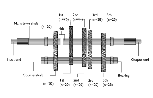
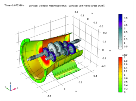
An external torque/load of 1000 Nm is applied at the output end of the drive shaft.
Part 2: Acoustics Analysis
Unidirectional Coupling
When coupling multibody/structural and acoustics physics, unidirectional coupling can be assumed if the exterior fluid is air (or any other light fluid). This implies that the vibrations from the gearbox housing affects the surrounding fluid, whereas the feedback from the acoustic waves to the structure is neglected. This model uses such an approach.
Time to Frequency FFT
The multibody dynamics is solved in the time domain, whereas the acoustics is solved in the frequency domain. Therefore the FFT solver is used to convert the housing accelerations from the time domain to the frequency domain.
Figure 3: The air domain surrounding the gearbox used in the acoustics analysis. The two microphone locations are also shown.
Domain Equations
This model solves the problem in the frequency domain using the Pressure Acoustics, Frequency Domain interface. The model equation is a slightly modified version of the Helmholtz equation for the acoustic pressure  p:
where ρ is the density, c is the speed of sound, and ω is the angular frequency.
Note: To reduce the computation time, linear elements are used in the discretization. To get more accurate results, quadratic elements can be used.
Boundary Conditions
The following boundary conditions are applied in the acoustic domain:
where an is the normal acceleration. The normal acceleration is applied only on those boundaries of the gearbox which are exposed to the air.
Model Parameters
The domain material is chosen as air. The following parameters are used in the model:
The excitation frequency band is taken as 1000 Hz to 3000 Hz in the steps of 20 Hz.
Frequency to Time FFT
After solving the acoustics problem for a range of frequencies, the results are transformed into the time domain using the FFT solver in order to visualize the transient wave propagation in the gearbox surrounding.
Sound Generation
After solving for the acoustics problem in the frequency domain, the pressure data of any location can be converted into a sound file. A Model Method is used for this purpose which requires the magnitude and phase of the pressure as a function of frequency.
Two microphones, as shown in Figure 3, are added at the following locations:
These are the default locations defined in the Parameters, and they can be changed as per the requirement.
Results and Discussion
The multibody dynamics analysis of the gearbox is performed in the time domain for one revolution of the main shaft. The von-Mises stress distribution in the housing at a particular instant is shown in Figure 4. The speed of different gears can also be seen in the figure.
Figure 4: von Mises stress distribution in the housing at t = 0.0754 s. The speed of different gears is also shown.
While gearbox is in operation, it starts vibrating under the influence of various forces. The normal acceleration of the housing, a measure of the noise radiation, is shown in Figure 5. This normal acceleration profile is plotted for a particular instance in time. So in order to understand the variation of normal acceleration with time, we can choose any one of the locations on the gearbox housing. The time history of normal acceleration of one of the points at the top of the gearbox is shown in Figure 6. In this figure, the normal acceleration is plotted with the rotation of the main shaft.
In order to have a better understanding about the frequency content, we can transform these results in the frequency domain by using the FFT solver as shown in Figure 7. It is clear from the plot that normal acceleration of the housing contains definitely more than one frequency. The frequency band in which the housing vibration is dominant is 1000 Hz to 3000 Hz.
Figure 5: Normal acceleration of the housing at t=0.0754 s. The speed of the different gears is also shown.
The sound pressure level in the near field as well as on the surface of the gearbox housing is shown in Figure 8 and Figure 9 respectively. The sound pressure level at far field in different planes can be seen in Figure 10, Figure 11, and Figure 12. These far-fields plots of sound pressure level give a clear idea about the directivity of noise radiation at a particular frequency.
Figure 6: Time history of the normal acceleration at one of the points at the top of the gearbox.
Figure 7: Frequency spectrum of the normal acceleration at one of the points at the top of the gearbox.
Figure 8: Sound pressure level outside the gearbox at 2000 Hz.
Figure 9: Sound pressure level at the surface of the gearbox at 2000 Hz.
Figure 10: Far-field sound pressure level at a distance of 1m in the xy-plane at 2000 Hz.
Figure 11: Far-field sound pressure level at a distance of 1m in the xz-plane at 2000 Hz.
Figure 12: Far-field sound pressure level at a distance of 1m in the yz-plane at 2000 Hz.
The pressure magnitude at two microphone locations as a function of frequency is shown in Figure 13. It can be seen that the magnitude of pressure at microphone 1 is higher than the second one as it is nearer to the source of noise.
In order to visualize the pressure wave propagation in the air domain outside the gearbox, the frequency domain pressure data can be converted back to the time domain. The pressure field at a particular instance in time is shown in Figure 14.
Figure 13: Frequency spectrum of the pressure magnitude at two microphone locations.
Figure 14: Total acoustics pressure field outside the gearbox at t=0.00377 s.
Notes About the COMSOL Implementation
Note: Model methods can only be set up in the COMSOL Desktop environment on the Windows version of COMSOL Multiphysics.
Application Library path: Acoustics_Module/Vibrations_and_FSI/gearbox_vibration_noise
Modeling Instructions
From the File menu, choose New.
New
In the New window, click  Model Wizard.
Model Wizard
1
In the Model Wizard window, click  3D.
2
In the Select Physics tree, select Structural Mechanics>Multibody Dynamics (mbd).
3
Click Add.
4
Click  Study.
5
In the Select Study tree, select General Studies>Time Dependent.
6
Geometry 1
Import 1 (imp1)
1
In the Home toolbar, click  Import.
2
In the Settings window for Import, locate the Import section.
3
Click Browse.
4
Form Union (fin)
1
In the Model Builder window, under Component 1 (comp1)>Geometry 1 click Form Union (fin).
2
In the Settings window for Form Union/Assembly, locate the Form Union/Assembly section.
3
From the Action list, choose Form an assembly.
4
Clear the Create pairs check box.
5
In the Home toolbar, click  Build All.
6
Click the  Click and Hide button in the Graphics toolbar.
7
Click the  Select Domains button in the Graphics toolbar.
8
On the object fin, select Domain 4 only.
9
Click the  Click and Hide button in the Graphics toolbar.
Global Definitions
Parameters 1
1
In the Model Builder window, under Global Definitions click Parameters 1.
2
In the Settings window for Parameters, locate the Parameters section.
3
Click  Load from File.
4
Definitions
Variables 1
1
In the Model Builder window, expand the Component 1 (comp1)>Definitions node.
2
Right-click Definitions and choose Variables.
3
In the Settings window for Variables, locate the Variables section.
4
Step 1 (step1)
1
In the Home toolbar, click  Functions and choose Global>Step.
2
In the Settings window for Step, locate the Parameters section.
3
In the Location text field, type T/40.
4
Click to expand the Smoothing section. In the Size of transition zone text field, type T/20.
Explicit 1
1
In the Definitions toolbar, click  Explicit.
2
In the Settings window for Explicit, locate the Input Entities section.
3
From the Geometric entity level list, choose Boundary.
4
Click  Paste Selection.
5
In the Paste Selection dialog box, type 367-370 in the Selection text field.
6
Explicit 2
1
Right-click Explicit 1 and choose Duplicate.
2
In the Settings window for Explicit, locate the Input Entities section.
3
Click  Clear Selection.
4
Click  Paste Selection.
5
In the Paste Selection dialog box, type 372-375, 377, 379-381 in the Selection text field.
6
Explicit 3
1
Right-click Explicit 2 and choose Duplicate.
2
In the Settings window for Explicit, locate the Input Entities section.
3
Click  Clear Selection.
4
Click  Paste Selection.
5
In the Paste Selection dialog box, type 818-821 in the Selection text field.
6
Explicit 4
1
Right-click Explicit 3 and choose Duplicate.
2
In the Settings window for Explicit, locate the Input Entities section.
3
Click  Clear Selection.
4
Click  Paste Selection.
5
In the Paste Selection dialog box, type 824-826, 828, 830, 832-834 in the Selection text field.
6
Explicit 5
1
Right-click Explicit 4 and choose Duplicate.
2
In the Settings window for Explicit, locate the Input Entities section.
3
Click  Clear Selection.
4
Click  Paste Selection.
5
In the Paste Selection dialog box, type 184-190, 193-209, 214-217, 226-240, 242-246, 533-540, 602-613, 677-680, 683-690 in the Selection text field.
6
Explicit 6
1
Right-click Explicit 5 and choose Duplicate.
2
In the Settings window for Explicit, locate the Input Entities section.
3
From the Geometric entity level list, choose Domain.
4
Click  Paste Selection.
5
In the Paste Selection dialog box, type 1-8 in the Selection text field.
6
7
In the Settings window for Explicit, locate the Output Entities section.
8
From the Output entities list, choose Adjacent boundaries.
General Extrusion 1 (genext1)
1
In the Definitions toolbar, click  Nonlocal Couplings and choose General Extrusion.
2
In the Settings window for General Extrusion, locate the Source Selection section.
3
From the Geometric entity level list, choose Boundary.
4
From the Selection list, choose Explicit 6.
Add Material
1
In the Home toolbar, click  Add Material to open the Add Material window.
2
Go to the Add Material window.
3
In the tree, select Built-in>Structural steel.
4
Click Add to Component in the window toolbar.
5
In the Home toolbar, click  Add Material to close the Add Material window.
Multibody Dynamics (mbd)
To start with, define the gears mounted on the counter shaft.
Helical Gear: Fourth (Counter Shaft)
1
In the Model Builder window, under Component 1 (comp1) right-click Multibody Dynamics (mbd) and choose Gears>Helical Gear.
2
3
In the Settings window for Helical Gear, type Helical Gear: Fourth (Counter Shaft) in the Label text field.
4
Locate the Gear Properties section. In the n text field, type n4i.
5
In the dp text field, type d4i.
6
In the α text field, type alpha.
7
In the β text field, type beta.
8
Locate the Gear Axis section. Specify the eg vector as
Helical Gears (Counter Shaft)
You can create the remaining helical gears mounted on the counter shaft by duplicating Helical Gear: Fourth (Counter Shaft) and resetting the information given in the table below:
Rigid Domain: Counter Shaft
1
In the Physics toolbar, click  Domains and choose Rigid Domain.
2
In the Settings window for Rigid Domain, type Rigid Domain: Counter Shaft in the Label text field.
3
Fixed Joint 1
1
In the Physics toolbar, click  Global and choose Fixed Joint.
2
In the Settings window for Fixed Joint, locate the Attachment Selection section.
3
From the Source list, choose Rigid Domain: Counter Shaft.
4
From the Destination list, choose Helical Gear: Fourth (Counter Shaft).
Fixed Joints
You can create the remaining fixed joints by duplicating Fixed Joint 1 and resetting the information given in the table below:
Now define the gears mounted on the main shaft.
Helical Gear: Fourth (Main Shaft)
1
In the Model Builder window, right-click Helical Gear: Fourth (Counter Shaft) and choose Duplicate.
2
In the Settings window for Helical Gear, type Helical Gear: Fourth (Main Shaft) in the Label text field.
3
Locate the Domain Selection section. Click  Clear Selection.
4
5
Locate the Gear Properties section. In the n text field, type n4o.
6
In the dp text field, type d4o.
7
In the β text field, type -beta.
Helical Gears (Main Shaft)
You can create the remaining helical gears mounted on the main shaft by duplicating Helical Gear: Fourth (Main Shaft) and resetting the information given in the table below:
Rigid Domain: Main Input Shaft
1
In the Physics toolbar, click  Domains and choose Rigid Domain.
2
In the Settings window for Rigid Domain, type Rigid Domain: Main Input Shaft in the Label text field.
3
Rigid Domain: Main Output Shaft
1
Right-click Rigid Domain: Main Input Shaft and choose Duplicate.
2
In the Settings window for Rigid Domain, type Rigid Domain: Main Output Shaft in the Label text field.
3
Locate the Domain Selection section. Click  Clear Selection.
4
Fixed Joint 6
1
In the Model Builder window, under Component 1 (comp1)>Multibody Dynamics (mbd) right-click Fixed Joint 5 and choose Duplicate.
2
In the Settings window for Fixed Joint, locate the Attachment Selection section.
3
From the Source list, choose Rigid Domain: Main Input Shaft.
4
From the Destination list, choose Helical Gear: Fourth (Main Shaft).
Hinge Joint 1
1
In the Physics toolbar, click  Global and choose Hinge Joint.
2
In the Settings window for Hinge Joint, locate the Attachment Selection section.
3
From the Source list, choose Rigid Domain: Main Output Shaft.
4
From the Destination list, choose Helical Gear: First (Main Shaft).
Prescribed Motion 1
1
In the Physics toolbar, click  Attributes and choose Prescribed Motion.
2
In the Settings window for Prescribed Motion, locate the Prescribed Rotational Motion section.
3
From the Activation condition list, choose Conditionally active.
4
In the iθp text field, type n!=1.
Hinge Joints
You can create the remaining hinge joints by duplicating Hinge Joint 1 and resetting the information given in the table below:
Hinge Joint 5
1
In the Model Builder window, click Hinge Joint 5.
2
In the Settings window for Hinge Joint, locate the Center of Joint section.
3
From the Entity level list, choose Point.
Center of Joint: Point 1
1
In the Model Builder window, click Center of Joint: Point 1.
2
In the Settings window for Center of Joint: Point, locate the Point Selection section.
3
Click  Paste Selection.
4
In the Paste Selection dialog box, type 151-152 in the Selection text field.
5
After defining all the gears, now define the gear connections.
Gear Pair: Fourth
1
In the Physics toolbar, click  Global and choose Gear Pair.
2
In the Settings window for Gear Pair, type Gear Pair: Fourth in the Label text field.
3
Locate the Gear Selection section. From the Wheel list, choose Helical Gear: Fourth (Main Shaft).
4
From the Pinion list, choose Helical Gear: Fourth (Counter Shaft).
5
Locate the Gear Pair Properties section. Select the Include gear elasticity check box.
Gear Elasticity 1
1
In the Model Builder window, click Gear Elasticity 1.
2
In the Settings window for Gear Elasticity, locate the Mesh Stiffness section.
3
In the kt,wh text field, type kt.
4
In the kt,pn text field, type kt.
5
From the Contact ratio in mesh cycle list, choose Varying.
6
In the ζ text field, type 0.8.
Gear Pairs
You can create the remaining gear pairs by duplicating Gear Pair: Fourth and resetting the information given in the table below:
Now define the connection between the shafts and the housing.
Attachment: Bearing 1 (Counter Shaft)
1
In the Physics toolbar, click  Boundaries and choose Attachment.
2
In the Settings window for Attachment, type Attachment: Bearing 1 (Counter Shaft) in the Label text field.
3
Locate the Boundary Selection section. From the Selection list, choose Explicit 1.
Attachments
You can create the remaining attachments by duplicating Attachment: Bearing 1 (Counter Shaft) and resetting the information given in the table below:
Hinge Joint 6
1
In the Physics toolbar, click  Global and choose Hinge Joint.
2
In the Settings window for Hinge Joint, locate the Attachment Selection section.
3
From the Source list, choose Attachment: Bearing 1 (Counter Shaft).
4
From the Destination list, choose Rigid Domain: Counter Shaft.
Hinge Joints
You can create the remaining hinge joints by duplicating Hinge Joint 6 and resetting the information given in the table below:
Hinge Joint 7
In the Model Builder window, click Hinge Joint 7.
Prescribed Motion 1
1
In the Physics toolbar, click  Attributes and choose Prescribed Motion.
2
In the Settings window for Prescribed Motion, locate the Prescribed Rotational Motion section.
3
From the Prescribed motion through list, choose Angular velocity.
4
In the ωp text field, type omega*step1(t[1/s]).
Hinge Joint 9
In the Model Builder window, click Hinge Joint 9.
Applied Force and Moment 1
1
In the Physics toolbar, click  Attributes and choose Applied Force and Moment.
2
In the Settings window for Applied Force and Moment, locate the Applied On section.
3
4
Locate the Applied Force and Moment section. In the M text field, type -T_ext*step1(t[1/s]).
Fixed Constraint 1
1
In the Physics toolbar, click  Boundaries and choose Fixed Constraint.
2
In the Settings window for Fixed Constraint, locate the Boundary Selection section.
3
From the Selection list, choose Explicit 5.
Study: Multibody Analysis
1
In the Model Builder window, click Study 1.
2
In the Settings window for Study, type Study: Multibody Analysis in the Label text field.
3
Locate the Study Settings section. Clear the Generate default plots check box.
Step 1: Time Dependent
1
In the Model Builder window, under Study: Multibody Analysis click Step 1: Time Dependent.
2
In the Settings window for Time Dependent, locate the Study Settings section.
3
In the Output times text field, type range(0,T/2000,T).
Solution 1 (sol1)
1
In the Study toolbar, click  Show Default Solver.
2
In the Model Builder window, expand the Solution 1 (sol1) node, then click Time-Dependent Solver 1.
3
In the Settings window for Time-Dependent Solver, click to expand the Time Stepping section.
4
From the Steps taken by solver list, choose Intermediate.
5
In the Study toolbar, click  Compute.
Results
In the Model Builder window, expand the Results node.
Study: Multibody Analysis/Solution 1 (2) (sol1)
1
In the Model Builder window, expand the Results>Datasets node.
2
Right-click Results>Datasets>Study: Multibody Analysis/Solution 1 (sol1) and choose Duplicate.
Selection
1
In the Results toolbar, click  Attributes and choose Selection.
2
In the Settings window for Selection, locate the Geometric Entity Selection section.
3
From the Geometric entity level list, choose Domain.
4
Click  Paste Selection.
5
In the Paste Selection dialog box, type 1-2, 8-18 in the Selection text field.
6
Study: Multibody Analysis/Solution 1 (3) (sol1)
In the Model Builder window, under Results>Datasets right-click Study: Multibody Analysis/Solution 1 (2) (sol1) and choose Duplicate.
Selection
1
In the Model Builder window, expand the Study: Multibody Analysis/Solution 1 (3) (sol1) node, then click Selection.
2
In the Settings window for Selection, locate the Geometric Entity Selection section.
3
Click  Clear Selection.
4
Click  Paste Selection.
5
In the Paste Selection dialog box, type 3, 5-7 in the Selection text field.
6
Follow the instructions below to plot the stress and normal acceleration in the housing as shown in Figure 4 and Figure 5 respectively.
Velocity - Stress
1
In the Results toolbar, click  3D Plot Group.
2
In the Settings window for 3D Plot Group, type Velocity - Stress in the Label text field.
Surface 1
1
Right-click Velocity - Stress and choose Surface.
2
In the Settings window for Surface, locate the Data section.
3
From the Dataset list, choose Study: Multibody Analysis/Solution 1 (2) (sol1).
4
Locate the Expression section. In the Expression text field, type mbd.vel.
5
Locate the Coloring and Style section. From the Color table list, choose AuroraAustralis.
Deformation 1
1
Right-click Surface 1 and choose Deformation.
2
In the Settings window for Deformation, locate the Scale section.
3
Select the Scale factor check box.
4
Surface 2
1
In the Model Builder window, under Results>Velocity - Stress right-click Surface 1 and choose Duplicate.
2
In the Settings window for Surface, locate the Data section.
3
From the Dataset list, choose Study: Multibody Analysis/Solution 1 (3) (sol1).
4
Locate the Expression section. In the Expression text field, type mbd.mises.
5
Locate the Coloring and Style section. From the Color table list, choose TrafficLight.
6
Click to expand the Range section. Select the Manual color range check box.
7
In the Minimum text field, type 0.
8
In the Maximum text field, type 2e7.
Velocity - Stress
1
In the Model Builder window, click Velocity - Stress.
2
In the Settings window for 3D Plot Group, locate the Color Legend section.
3
From the Position list, choose Right double.
4
In the Velocity - Stress toolbar, click  Plot.
5
Click the  Zoom Extents button in the Graphics toolbar.
Velocity - Normal Acceleration
1
Right-click Velocity - Stress and choose Duplicate.
2
In the Model Builder window, click Velocity - Stress 1.
3
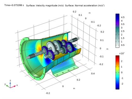
In the Settings window for 3D Plot Group, type Velocity - Normal Acceleration in the Label text field.
Surface 2
1
In the Model Builder window, expand the Results>Velocity - Normal Acceleration>Surface 2 node, then click Surface 2.
2
In the Settings window for Surface, locate the Expression section.
3
In the Expression text field, type an.
4
Locate the Range section. Clear the Manual color range check box.
5
Locate the Coloring and Style section. From the Color table list, choose Rainbow.
6
In the Velocity - Normal Acceleration toolbar, click  Plot.
7
Click the  Zoom Extents button in the Graphics toolbar.
Follow the instructions below to plot the time history and frequency spectrum of normal acceleration as shown in Figure 6 and Figure 7 respectively.
Normal Acceleration
1
In the Home toolbar, click  Add Plot Group and choose 1D Plot Group.
2
In the Settings window for 1D Plot Group, type Normal Acceleration in the Label text field.
Point Graph 1
1
Right-click Normal Acceleration and choose Point Graph.
2
In the Settings window for Point Graph, locate the Selection section.
3
Click  Paste Selection.
4
In the Paste Selection dialog box, type 879 in the Selection text field.
5
6
In the Settings window for Point Graph, locate the y-Axis Data section.
7
In the Expression text field, type an.
8
Locate the x-Axis Data section. From the Parameter list, choose Expression.
9
In the Expression text field, type mbd.hgj7.th.
10
From the Unit list, choose °.
11
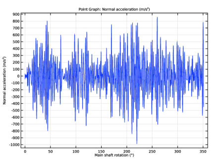
Select the Description check box.
12
13
In the Normal Acceleration toolbar, click  Plot.
14
Click the  Zoom Extents button in the Graphics toolbar.
Normal Acceleration: Frequency
1
In the Model Builder window, right-click Normal Acceleration and choose Duplicate.
2
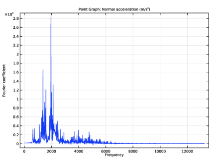
In the Settings window for 1D Plot Group, type Normal Acceleration: Frequency in the Label text field.
Point Graph 1
1
In the Model Builder window, expand the Normal Acceleration: Frequency node, then click Point Graph 1.
2
In the Settings window for Point Graph, locate the x-Axis Data section.
3
From the Parameter list, choose Frequency spectrum.
4
In the Normal Acceleration: Frequency toolbar, click  Plot.
5
Click the  Zoom Extents button in the Graphics toolbar.
Now add acoustics in the model for computing the noise radiation from the gearbox.
Add Component
In the Model Builder window, right-click the root node and choose Add Component>3D.
Geometry 2
1
In the Settings window for Geometry, locate the Advanced section.
2
From the Geometry representation list, choose CAD kernel.
Import 1 (imp1)
1
In the Home toolbar, click  Import.
2
In the Settings window for Import, locate the Import section.
3
Click Browse.
4
Convert to Solid 1 (csol1)
1
In the Geometry toolbar, click  Conversions and choose Convert to Solid.
2
Click in the Graphics window and then press Ctrl+A to select all objects.
Sphere 1 (sph1)
1
In the Geometry toolbar, click  Sphere.
2
In the Settings window for Sphere, locate the Size section.
3
In the Radius text field, type R.
Difference 1 (dif1)
1
In the Geometry toolbar, click  Booleans and Partitions and choose Difference.
2
3
In the Settings window for Difference, locate the Difference section.
4
Find the Objects to subtract subsection. Select the  Activate Selection toggle button.
5
Form Union (fin)
1
In the Geometry toolbar, click  Build All.
2
Click the  Zoom Extents button in the Graphics toolbar.
3
Click the  Click and Hide button in the Graphics toolbar.
4
Click the  Select Boundaries button in the Graphics toolbar.
5
In the Model Builder window, click Form Union (fin).
6
On the object fin, select Boundary 2 only.
7
Click the  Click and Hide button in the Graphics toolbar.
Definitions (comp2)
Explicit 7
1
In the Model Builder window, expand the Component 2 (comp2)>Definitions node.
2
Right-click Component 2 (comp2)>Definitions and choose Selections>Explicit.
3
In the Settings window for Explicit, locate the Input Entities section.
4
From the Geometric entity level list, choose Boundary.
5
Click  Paste Selection.
6
In the Paste Selection dialog box, type 1-4, 349-350, 357, 360 in the Selection text field.
7
Explicit 8
1
In the Definitions toolbar, click  Explicit.
2
In the Settings window for Explicit, locate the Input Entities section.
3
From the Geometric entity level list, choose Boundary.
4
Click  Paste Selection.
5
In the Paste Selection dialog box, type 12-20, 23-40, 43-47, 49, 53-73, 127, 132-134, 139, 144-193, 196-202, 205-207, 210-220, 223-229, 232-234, 237-244, 280-297, 299-318, 320-348, 351-356, 358-359, 361-681, 711-712, 715-720, 723-724, 727-734 in the Selection text field.
6
Add Material
1
In the Home toolbar, click  Add Material to open the Add Material window.
2
Go to the Add Material window.
3
4
Click Add to Component in the window toolbar.
5
In the Home toolbar, click  Add Material to close the Add Material window.
Add Physics
1
In the Home toolbar, click  Add Physics to open the Add Physics window.
2
Go to the Add Physics window.
3
In the tree, select Acoustics>Pressure Acoustics>Pressure Acoustics, Frequency Domain (acpr).
4
Find the Physics interfaces in study subsection. In the table, clear the Solve check box for Study: Multibody Analysis.
5
Click Add to Component 2 in the window toolbar.
6
In the Home toolbar, click  Add Physics to close the Add Physics window.
Pressure Acoustics, Frequency Domain (acpr)
1
In the Settings window for Pressure Acoustics, Frequency Domain, click to expand the Discretization section.
2
From the Element order list, choose Linear.
Spherical Wave Radiation 1
1
Right-click Component 2 (comp2)>Pressure Acoustics, Frequency Domain (acpr) and choose Radiation Conditions>Spherical Wave Radiation.
2
In the Settings window for Spherical Wave Radiation, locate the Boundary Selection section.
3
From the Selection list, choose Explicit 7.
Exterior Field Calculation 1
1
In the Physics toolbar, click  Boundaries and choose Exterior Field Calculation.
2
In the Settings window for Exterior Field Calculation, locate the Boundary Selection section.
3
From the Selection list, choose Explicit 7.
4
Click the  Show More Options button in the Model Builder toolbar.
5
In the Show More Options dialog box, in the tree, select the check box for the node Physics>Advanced Physics Options.
6
7
In the Settings window for Exterior Field Calculation, click to expand the Advanced Settings section.
8
Clear the Use polynomial-preserving recovery for the normal gradient check box.
Normal Acceleration 1
1
In the Physics toolbar, click  Boundaries and choose Normal Acceleration.
2
In the Settings window for Normal Acceleration, locate the Boundary Selection section.
3
From the Selection list, choose Explicit 8.
4
Locate the Normal Acceleration section. From the Type list, choose Acceleration.
5
Specify the a0 vector as
Mesh 2
1
In the Model Builder window, under Component 2 (comp2) click Mesh 2.
2
In the Settings window for Mesh, locate the Mesh Settings section.
3
From the Sequence type list, choose User-controlled mesh.
Size
1
In the Model Builder window, under Component 2 (comp2)>Mesh 2 click Size.
2
In the Settings window for Size, locate the Element Size section.
3
Click the Custom button.
4
Locate the Element Size Parameters section. In the Maximum element size text field, type 343/3000/4.
Boundary Layers 1
In the Mesh toolbar, click  Boundary Layers.
Boundary Layer Properties
1
In the Model Builder window, click Boundary Layer Properties.
2
In the Settings window for Boundary Layer Properties, locate the Geometric Entity Selection section.
3
From the Selection list, choose Explicit 7.
4
Locate the Boundary Layer Properties section. From the Thickness of first layer list, choose Manual.
5
In the Thickness text field, type 343/3000/4/10.
Add Study
1
In the Home toolbar, click  Add Study to open the Add Study window.
2
Go to the Add Study window.
3
Find the Studies subsection. In the Select Study tree, select Empty Study.
4
Click Add Study in the window toolbar.
5
In the Home toolbar, click  Add Study to close the Add Study window.
Study: Acoustics (Frequency Domain)
1
In the Settings window for Study, locate the Study Settings section.
2
Clear the Generate default plots check box.
3
In the Label text field, type Study: Acoustics (Frequency Domain).
Time to Frequency FFT
1
In the Study toolbar, click  Study Steps and choose Frequency Domain>Time to Frequency FFT.
2
In the Settings window for Time to Frequency FFT, locate the Study Settings section.
3
From the Input study list, choose Study: Multibody Analysis, Time Dependent.
4
In the End time text field, type T.
5
In the Maximum output frequency text field, type 250/T.
6
Locate the Physics and Variables Selection section. In the table, clear the Solve for check box for Pressure Acoustics, Frequency Domain (acpr).
Step 2: Frequency Domain
1
In the Model Builder window, right-click Study: Acoustics (Frequency Domain) and choose Study Steps>Frequency Domain>Frequency Domain.
2
In the Settings window for Frequency Domain, locate the Study Settings section.
3
In the Frequencies text field, type range(1000,20,3000).
4
Locate the Physics and Variables Selection section. In the table, clear the Solve for check box for Multibody Dynamics (mbd).
5
Click to expand the Values of Dependent Variables section. Find the Values of variables not solved for subsection. From the Settings list, choose User controlled.
6
From the Method list, choose Solution.
7
From the Study list, choose Study: Acoustics (Frequency Domain), Time to Frequency FFT.
8
From the Selection list, choose All.
Solution 2 (sol2)
1
In the Study toolbar, click  Show Default Solver.
2
In the Model Builder window, expand the Solution 2 (sol2) node.
3
In the Model Builder window, expand the Study: Acoustics (Frequency Domain)>Solver Configurations>Solution 2 (sol2)>Dependent Variables 2 node, then click Pressure (comp2.p).
4
In the Settings window for Field, locate the Scaling section.
5
From the Method list, choose Manual.
6
In the Scale text field, type 1e5.
7
In the Model Builder window, click Stationary Solver 1.
8
In the Settings window for Stationary Solver, locate the General section.
9
From the Linearity list, choose Linear.
10
In the Study toolbar, click  Compute.
Results
Study: Acoustics (Frequency Domain)/Solution 2 (6) (sol2)
In the Model Builder window, under Results>Datasets right-click Study: Acoustics (Frequency Domain)/Solution 2 (5) (sol2) and choose Duplicate.
Selection
1
In the Model Builder window, right-click Study: Acoustics (Frequency Domain)/Solution 2 (6) (sol2) and choose Selection.
2
In the Settings window for Selection, locate the Geometric Entity Selection section.
3
From the Geometric entity level list, choose Boundary.
4
From the Selection list, choose Explicit 8.
Follow the instructions below to plot the sound pressure level in the near field, housing surface, and the far field as shown in Figure 8, Figure 9, Figure 10, Figure 11 and Figure 12 respectively.
SPL Near Field
1
In the Results toolbar, click  3D Plot Group.
2
In the Settings window for 3D Plot Group, locate the Data section.
3
From the Dataset list, choose Study: Acoustics (Frequency Domain)/Solution 2 (5) (sol2).
4
From the Parameter value (freq (Hz)) list, choose 2000.
5
In the Label text field, type SPL Near Field.
Slice 1
1
Right-click SPL Near Field and choose Slice.
2
In the Settings window for Slice, locate the Expression section.
3
In the Expression text field, type acpr.Lp_t.
4
Locate the Plane Data section. In the Planes text field, type 1.
Slice 2
1
Right-click Slice 1 and choose Duplicate.
2
In the Settings window for Slice, click to expand the Title section.
3
From the Title type list, choose None.
4
Locate the Plane Data section. From the Plane list, choose ZX-planes.
5
In the Planes text field, type 1.
6
Click to expand the Inherit Style section. From the Plot list, choose Slice 1.
Slice 3
1
Right-click Slice 2 and choose Duplicate.
2
In the Settings window for Slice, locate the Plane Data section.
3
From the Plane list, choose XY-planes.
4
In the Planes text field, type 1.
5
In the SPL Near Field toolbar, click  Plot.
6
Click the  Zoom Extents button in the Graphics toolbar.
SPL Casing Surface
1
In the Home toolbar, click  Add Plot Group and choose 3D Plot Group.
2
In the Settings window for 3D Plot Group, locate the Data section.
3
From the Dataset list, choose Study: Acoustics (Frequency Domain)/Solution 2 (6) (sol2).
4
From the Parameter value (freq (Hz)) list, choose 2000.
5
In the Label text field, type SPL Casing Surface.
Surface 1
1
Right-click SPL Casing Surface and choose Surface.
2
In the Settings window for Surface, locate the Expression section.
3
In the Expression text field, type acpr.Lp_t.
4
In the SPL Casing Surface toolbar, click  Plot.
5
Click the  Zoom Extents button in the Graphics toolbar.
Polar SPL xy-plane
1
In the Home toolbar, click  Add Plot Group and choose Polar Plot Group.
2
In the Settings window for Polar Plot Group, type Polar SPL xy-plane in the Label text field.
3
Locate the Data section. From the Dataset list, choose Study: Acoustics (Frequency Domain)/Solution 2 (5) (sol2).
4
From the Parameter selection (freq) list, choose From list.
5
In the Parameter values (freq (Hz)) list, select 2000.
6
Click to expand the Title section. From the Title type list, choose Manual.
7
In the Title text area, type Sound Pressure Level - Exterior Field (xy-plane) (dB).
Radiation Pattern 1
1
In the Polar SPL xy-plane toolbar, click  More Plots and choose Radiation Pattern.
2
In the Settings window for Radiation Pattern, locate the Evaluation section.
3
Find the Angles subsection. In the Number of angles text field, type 360.
4
Click to expand the Coloring and Style section. In the Width text field, type 2.
5
In the Polar SPL xy-plane toolbar, click  Plot.
6
Click the  Zoom Extents button in the Graphics toolbar.
Polar SPL xz-plane
1
In the Model Builder window, right-click Polar SPL xy-plane and choose Duplicate.
2
In the Settings window for Polar Plot Group, type Polar SPL xz-plane in the Label text field.
3
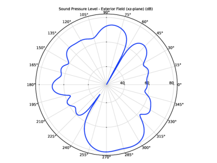
Locate the Title section. In the Title text area, type Sound Pressure Level - Exterior Field (xz-plane) (dB).
Radiation Pattern 1
1
In the Model Builder window, expand the Polar SPL xz-plane node, then click Radiation Pattern 1.
2
In the Settings window for Radiation Pattern, locate the Evaluation section.
3
Find the Normal vector subsection. In the y text field, type 1.
4
In the z text field, type 0.
5
In the Polar SPL xz-plane toolbar, click  Plot.
6
Click the  Zoom Extents button in the Graphics toolbar.
Polar SPL yz-plane
1
In the Model Builder window, right-click Polar SPL xz-plane and choose Duplicate.
2
In the Settings window for Polar Plot Group, type Polar SPL yz-plane in the Label text field.
3
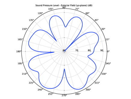
Locate the Title section. In the Title text area, type Sound Pressure Level - Exterior Field (yz-plane) (dB).
Radiation Pattern 1
1
In the Model Builder window, expand the Polar SPL yz-plane node, then click Radiation Pattern 1.
2
In the Settings window for Radiation Pattern, locate the Evaluation section.
3
Find the Normal vector subsection. In the x text field, type 1.
4
In the y text field, type 0.
5
In the Polar SPL yz-plane toolbar, click  Plot.
6
Click the  Zoom Extents button in the Graphics toolbar.
Now first define the microphone locations and then evaluate the pressure on those locations. Also plot the microphone pressure as shown in Figure 13.
Parameters
1
In the Results toolbar, click  Parameters.
2
In the Settings window for Parameters, locate the Parameters section.
3
Click  Load from File.
4
Global Evaluation: Microphone 1
1
In the Results toolbar, click  Global Evaluation.
2
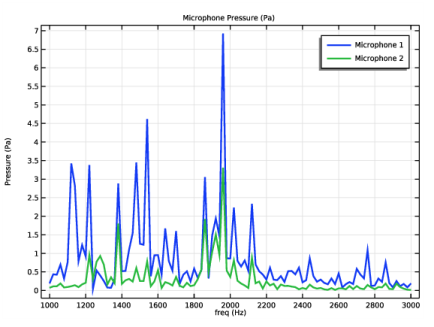
In the Settings window for Global Evaluation, type Global Evaluation: Microphone 1 in the Label text field.
3
Locate the Data section. From the Dataset list, choose Study: Acoustics (Frequency Domain)/Solution 2 (5) (sol2).
4
Locate the Expressions section. In the table, enter the following settings:
5
Click  Evaluate.
Table
Go to the Table window.
Global Evaluation: Microphone 2
1
Right-click Global Evaluation: Microphone 1 and choose Duplicate.
2
In the Settings window for Global Evaluation, type Global Evaluation: Microphone 2 in the Label text field.
3
Locate the Expressions section. In the table, enter the following settings:
4
Clicknext to  Evaluate, then choose New Table.
Microphone Pressure
1
In the Results toolbar, click  1D Plot Group.
2
In the Settings window for 1D Plot Group, type Microphone Pressure in the Label text field.
3
Locate the Data section. From the Dataset list, choose Study: Acoustics (Frequency Domain)/Solution 2 (5) (sol2).
4
Click to expand the Title section. From the Title type list, choose Manual.
5
In the Title text area, type Microphone Pressure (Pa).
6
Locate the Plot Settings section. Select the y-axis label check box.
7
Global 1
1
Right-click Microphone Pressure and choose Global.
2
In the Settings window for Global, locate the y-Axis Data section.
3
4
Click to expand the Coloring and Style section. In the Width text field, type 2.
5
In the Microphone Pressure toolbar, click  Plot.
6
Click the  Zoom Extents button in the Graphics toolbar.
Follow the instructions below to convert the pressure data from frequency domain to time domain and plot the pressure field in the gearbox surrounding as shown in Figure 14.
Add Study
1
In the Home toolbar, click  Add Study to open the Add Study window.
2
Go to the Add Study window.
3
Find the Studies subsection. In the Select Study tree, select Empty Study.
4
Click Add Study in the window toolbar.
5
In the Home toolbar, click  Add Study to close the Add Study window.
Study: Acoustics (Time Domain)
1
In the Settings window for Study, type Study: Acoustics (Time Domain) in the Label text field.
2
Locate the Study Settings section. Clear the Generate default plots check box.
Frequency to Time FFT
1
In the Study toolbar, click  Study Steps and choose Time Dependent>Frequency to Time FFT.
2
In the Settings window for Frequency to Time FFT, locate the Study Settings section.
3
In the Times text field, type range(0,T/2000,T/20).
4
From the Input study list, choose Study: Acoustics (Frequency Domain), Frequency Domain.
5
Locate the Physics and Variables Selection section. In the table, clear the Solve for check box for Multibody Dynamics (mbd).
6
In the Study toolbar, click  Compute.
Results
Pressure Near Field: Time
1
In the Home toolbar, click  Add Plot Group and choose 3D Plot Group.
2
In the Settings window for 3D Plot Group, type Pressure Near Field: Time in the Label text field.
3
Locate the Data section. From the Dataset list, choose Study: Acoustics (Time Domain)/Solution 3 (8) (sol3).
Slice 1
1
In the Model Builder window, expand the Pressure Near Field: Time node.
2
Right-click Pressure Near Field: Time and choose Slice.
3
In the Settings window for Slice, locate the Plane Data section.
4
In the Planes text field, type 1.
5
Locate the Coloring and Style section. From the Color table list, choose Wave.
Slice 2
1
Right-click Slice 1 and choose Duplicate.
2
In the Settings window for Slice, locate the Title section.
3
From the Title type list, choose None.
4
Locate the Plane Data section. From the Plane list, choose ZX-planes.
5
In the Planes text field, type 1.
6
Locate the Inherit Style section. From the Plot list, choose Slice 1.
Slice 3
1
Right-click Slice 2 and choose Duplicate.
2
In the Settings window for Slice, locate the Plane Data section.
3
From the Plane list, choose XY-planes.
4
In the Planes text field, type 1.
Filter 1
1
In the Model Builder window, right-click Slice 1 and choose Filter.
2
In the Settings window for Filter, locate the Element Selection section.
3
In the Logical expression for inclusion text field, type y>0.
Filter 1
1
In the Model Builder window, right-click Slice 2 and choose Filter.
2
In the Settings window for Filter, locate the Element Selection section.
3
In the Logical expression for inclusion text field, type x>0.
4
In the Pressure Near Field: Time toolbar, click  Plot.
5
Click the  Zoom Extents button in the Graphics toolbar.
Create animations to visualize the gearbox vibration and the propagation of the sound wave in the surrounding.
Animation 1
1
In the Results toolbar, click  Animation and choose Player.
2
In the Settings window for Animation, locate the Frames section.
3
In the Number of frames text field, type 50.
Animation 2
1
Right-click Animation 1 and choose Duplicate.
2
In the Settings window for Animation, locate the Scene section.
3
From the Subject list, choose Velocity - Normal Acceleration.
Animation 3
1
Right-click Animation 2 and choose Duplicate.
2
In the Settings window for Animation, locate the Scene section.
3
From the Subject list, choose Pressure Near Field: Time.
Create Model Methods in order to convert the pressure data evaluated at microphone locations into sound files.
New Method
1
In the Developer toolbar, click  New Method.
2
In the New Method dialog box, type Microphone1 in the Name text field.
3
Application Builder
Microphone1
1
In the Application Builder window, under Methods click Microphone1.
2
// This method is to play the sound at microphone 1.
// It uses absolute value and phase of pressure field as a function of frequency.

if (!model.sol("sol2").isEmpty()) {

// Evaluate absolute pressure and phase at the given location as a function of frequency.
model.result().numerical("gev1").setResult();
double[] pressureAbs = model.result().numerical("gev1").getReal()[0];
double[] pressurePhase = model.result().numerical("gev1").getReal()[1];
double[] freq = model.result().numerical("gev1").getReal()[2];

// Convert pressure data into a sound file.
try {
// Set the number of samples in the highest frequency wave and the total audio time in seconds.
int n = 20;
int time = 4;

float sampleRate = (float) freq[freq.length-1]*n;
byte buffer[] = new byte[(int) sampleRate*2*time];

// Use ShortBuffer (signed 16-bit with big-endian byte order) and ByteBuffer for easily adding new bytes to the buffer.
java.nio.ByteBuffer byteBuffer = java.nio.ByteBuffer.wrap(buffer);
java.nio.ShortBuffer shortBuffer = byteBuffer.asShortBuffer();

// Set up AudioFormat, DataLine, and SourceDataLine in order to play sound with the Java sound API.
javax.sound.sampled.AudioFormat audioFormat = new javax.sound.sampled.AudioFormat(sampleRate, 16, 1, true, true);

int bytesPerSample = 2;
for (int i = 0; i < buffer.length/bytesPerSample; i++) {
double t = i/sampleRate;
// Add the six components and divide by the sum of the amplitude of the signals.
double amplitude = 0;

for (int j = 0; j < pressureAbs.length; j++) {
amplitude += pressureAbs[j]*Math.sin(2*Math.PI*freq[j]*t+pressurePhase[j]);
}

// Multiply the signal with 1200 in order to get a decent volume on the envelope signal.
shortBuffer.put((short) (1200*amplitude));
}
java.io.ByteArrayInputStream byteArrayInputStream = new java.io.ByteArrayInputStream(buffer);

// Write to the file in order to create the file.
writeFile("temp:///gearbox_vibration_noise_mic1.wav", "");
// Get the absolute file path of the generated temp file for the wave output.
String tempWaveFilePath = getFilePath("temp:///gearbox_vibration_noise_mic1.wav");
java.io.File waveFile = null;
if (tempWaveFilePath != null) {
waveFile = new java.io.File(tempWaveFilePath); // Create a File instance.
}
// Create an input stream taking the byte[] buffer.
javax.sound.sampled.AudioInputStream audioInputStream = new javax.sound.sampled.AudioInputStream(byteArrayInputStream, audioFormat, buffer.length/audioFormat.getFrameSize());

// Write the audio input stream of the sound buffer to the wave file and play the wave file.
// A wave file is used instead of directly playing to a source data line for the sound device on
// the computer because of the client user interface may run on another machine.
// playSound functionality ensures the sound is always played for the client user interface.
if (waveFile != null) {
javax.sound.sampled.AudioSystem.write(audioInputStream, javax.sound.sampled.AudioFileFormat.Type.WAVE, waveFile);
playSound("temp:///gearbox_vibration_noise_mic1.wav");
}

} catch (Exception ex) {
debugLog(ex.getMessage());
error("Error when creating fundamental and harmonics sound combination.");
}
}
New Method
1
In the Developer toolbar, click  New Method.
2
In the New Method dialog box, type Microphone2 in the Name text field.
3
Microphone2
1
In the Application Builder window, under Methods click Microphone2.
2
// This method is to play the sound at microphone 2.
// It uses absolute value and phase of pressure field as a function of frequency.

if (!model.sol("sol2").isEmpty()) {

// Evaluate absolute pressure and phase at the given location as a function of frequency.
model.result().numerical("gev2").setResult();
double[] pressureAbs = model.result().numerical("gev2").getReal()[0];
double[] pressurePhase = model.result().numerical("gev2").getReal()[1];
double[] freq = model.result().numerical("gev2").getReal()[2];

// Convert pressure data into a sound file.
try {
// Set the number of samples in the highest frequency wave and the total audio time in seconds.
int n = 20;
int time = 4;

float sampleRate = (float) freq[freq.length-1]*n;
byte buffer[] = new byte[(int) sampleRate*2*time];

// Use ShortBuffer (signed 16-bit with big-endian byte order) and ByteBuffer for easily adding new bytes to the buffer.
java.nio.ByteBuffer byteBuffer = java.nio.ByteBuffer.wrap(buffer);
java.nio.ShortBuffer shortBuffer = byteBuffer.asShortBuffer();

// Set up AudioFormat, DataLine, and SourceDataLine in order to play sound with the Java sound API.
javax.sound.sampled.AudioFormat audioFormat = new javax.sound.sampled.AudioFormat(sampleRate, 16, 1, true, true);

int bytesPerSample = 2;
for (int i = 0; i < buffer.length/bytesPerSample; i++) {
double t = i/sampleRate;
// Add the six components and divide by the sum of the amplitude of the signals.
double amplitude = 0;

for (int j = 0; j < pressureAbs.length; j++) {
amplitude += pressureAbs[j]*Math.sin(2*Math.PI*freq[j]*t+pressurePhase[j]);
}

// Multiply the signal with 1200 in order to get a decent volume on the envelope signal.
shortBuffer.put((short) (1200*amplitude));
}
java.io.ByteArrayInputStream byteArrayInputStream = new java.io.ByteArrayInputStream(buffer);

// Write to the file in order to create the file.
writeFile("temp:///gearbox_vibration_noise_mic2.wav", "");
// Get the absolute file path of the generated temp file for the wave output.
String tempWaveFilePath = getFilePath("temp:///gearbox_vibration_noise_mic2.wav");
java.io.File waveFile = null;
if (tempWaveFilePath != null) {
waveFile = new java.io.File(tempWaveFilePath); // Create a File instance.
}
// Create an input stream taking the byte[] buffer.
javax.sound.sampled.AudioInputStream audioInputStream = new javax.sound.sampled.AudioInputStream(byteArrayInputStream, audioFormat, buffer.length/audioFormat.getFrameSize());

// Write the audio input stream of the sound buffer to the wave file and play the wave file.
// A wave file is used instead of directly playing to a source data line for the sound device on
//the computer because of the client user interface may run on another machine.
// playSound functionality ensures the sound is always played for the client user interface.
if (waveFile != null) {
javax.sound.sampled.AudioSystem.write(audioInputStream, javax.sound.sampled.AudioFileFormat.Type.WAVE, waveFile);
playSound("temp:///gearbox_vibration_noise_mic2.wav");
}

} catch (Exception ex) {
debugLog(ex.getMessage());
error("Error when creating fundamental and harmonics sound combination.");
}
}
Methods
In the Home toolbar, click  Model Builder.
Global Definitions
Click  Method Call and choose Microphone1.
Microphone1
1
In the Model Builder window, under Global Definitions right-click Microphone1 and choose Run.
2
In the Home toolbar, click  Run Method Call and choose Microphone1.
3
Click  Method Call and choose Microphone2.
Microphone2
1
In the Model Builder window, right-click Microphone2 and choose Run.
2
In the Home toolbar, click  Run Method Call and choose Microphone2.
Results
Thumbnail
1
In the Model Builder window, right-click Velocity - Stress and choose Duplicate.
2
In the Model Builder window, click Velocity - Stress 1.
3
In the Settings window for 3D Plot Group, type Thumbnail in the Label text field.
Isosurface 1
1
Right-click Thumbnail and choose Isosurface.
2
In the Settings window for Isosurface, locate the Data section.
3
From the Dataset list, choose Study: Acoustics (Frequency Domain)/Solution 2 (5) (sol2).
4
From the Parameter value (freq (Hz)) list, choose 1300.
5
Locate the Expression section. In the Expression text field, type acpr.Lp_t.
6
Locate the Levels section. In the Total levels text field, type 10.
Filter 1
1
Right-click Isosurface 1 and choose Filter.
2
In the Settings window for Filter, locate the Element Selection section.
3
In the Logical expression for inclusion text field, type y>0.1.
4
In the Thumbnail toolbar, click  Plot.