PDF

Axisymmetric Condenser Microphone with Electrical Lumping
Introduction
This is a model of a condenser microphone with a simple axisymmetric geometry. The model aims to give a precise description of the physical working principles of such a microphone, using lumped descriptions for some of the physical phenomena. Lumping certain parts of a model can give additional insight to physical phenomena using a simplified description. A fully coupled approach (without lumping internal physics) can be seen in the Axisymmetric Condenser Microphone model, also located in the Application Library of the Acoustics Module.
The condenser microphone is considered to be the microphone with highest quality when performing precise acoustical measurements and with high-fidelity reproduction properties when performing sound recordings, see Ref. 2. This electromechanical acoustic transducer works by transforming the mechanical deformation of a thin membrane (diaphragm) into an AC voltage signal.
Figure 1: Sketch of the condenser microphone system including variables and coordinate system. The red box indicates the modeled region.
Models for describing condenser microphones have classically been of the equivalent network type (see Ref. 2). Analytical models exist for simpler geometries, but there are also highly advanced analytical models for more complex geometries; see for example Ref. 1. In the present detailed finite-element (FE) model, you model the microphone including a static (quiescent) analysis of the DC charging (prepolarization) and deformation of the membrane. You then perform time-harmonic (small-signal) finite element (FE) analysis of the dynamics of the membrane coupled to thermoviscous acoustics. The small-signal electric model for the system is solved as a lumped (electric equivalent) model coupled to the FE model. The model is a true multiphysics problem that involves several physics interfaces: Thermoviscous Acoustics, Electrostatics, Moving Mesh, two user-defined PDE interfaces, a Global ODEs and DAEs interface, as well as an Electrical Circuit model.
Note: This application requires the AC/DC Module.
Model Definition
The geometry and model definitions are shown in Figure 1. The membrane is deformed due to the electrostatic forces from charging the capacitor and because of the pressure variation from the external incoming uniform acoustic signal pin. The chosen dimensions of the microphone are typical generic dimensions. Dimensions and parameters are given in Table 1.
Hm
18 μm
Rmem
54 μm
Tm
tm
7 μm
ρm
Vpol
The membrane is backed by a thin air gap of thickness Hm and a back electrode. Because the gap is so small, the inclusion of thermal and viscous losses in the acoustic model is essential, thus using the thermoviscous acoustics interface. The membrane and back electrode makes up a capacitor that is polarized by an external DC voltage source. The air gap acts as a damping layer for the membrane vibrations. As the gap between the membrane and the back electrode varies a voltage change is induced and is coupled to the capacitor (the quiescent DC capacitance of the system C0) and an external very large resistive load RL.
The electric circuit for this coupling is shown in Figure 2.
Figure 2: Analogous circuit for the electrical part of the condenser microphone.
The sensitivity L of the condenser microphone is measured in the unit dB (relative to 1 V/Pa). It is defined as the ratio of the open circuit output voltage Vout to the input pressure pin and is given by
Next, consider a small-signal (linearized) analysis of the electric part of the condenser microphone. The total voltage is the sum of the quiescent polarization voltage Vpol and the small-signal output voltage Vout. The total charge on the condenser is the sum of the quiescent charge Q and the small-signal charge q. The distance between the back electrode and the membrane is the sum of the initial distance Hm, the quiescent average deformation U0,av and the small-signal deformation Uav.
The capacitance C of a parallel plate capacitor, with a fixed air gap distance h and area A is given by
If the air gap h is varied with an average deformation Uav around the initial static gap distance, Hm + U0,av, the expression becomes
(1)
where the expression has been expanded to first order. Again, the distance U0,av stems from the initial deformation from equilibrium due to the electrostatic forces of the prepolarization of the condenser. A first approximation for the average deformation in axisymmetric coordinates is given as
(2)
The capacitance is by its definition (see Ref. 4) given by
(3)
where Q is the charge on and V the potential across the capacitor. Inserting Equation 1 into Equation 3 and retaining only first-order terms yields
(4)
Differentiating Equation 4 with respect to time, switching to frequency domain, and using Vpol = Q/C0 yields
(5)
where Icap is the induced current through the capacitor, the second term on the right is the electromechanical coupling Vcap, and the average membrane velocity is
(6)
where um is the axial membrane velocity. The circuit model equivalent to equation Equation 5 is shown in Figure 2.The governing equation of the membrane is described in the next section, Membrane Model. The final element necessary to couple the lumped small parameter model of the electric model to the mechanical FE model is the back coupling via the small parameter electrostatic force fes. The force is approximated by the spatial derivative (z direction) of the electric energy stored in a parallel plate condenser; the small parameter component is (see Ref. 2)
The force is applied evenly over the membrane as a surface normal stress .
Note that the integrals in Equation 2 and Equation 6 are over the area of the membrane that is backed by the back electrode plus a possible small correction for edge effects. This is especially important if the back electrode has holes. This is the case in many commercials condenser microphones where the holes are placed in order to produce a special sensitivity characteristic of the microphone. In this model the back electrode is flat and uniform.
Membrane Model
The displacement U of a thin axisymmetric membrane of thickness tm, under constant tension Tm, and with a density ρm is governed by the following equation
(7)
where r is the radial coordinate, t is time, ρms = ρm/tm is the surface density, and Fs is the sum of surface forces; see for example Ref. 3. In the present model, the surface force is the sum of the external incident pressure pin (it is assumed to be uniform over the microphone membrane), the internal pressure p = p(r) (given by the thermoviscous acoustics model), and the electrostatic force which is the sum of the quiescent Maxwell surface stress (given by the electrostatic model) and the small-signal force fes. The variations of the deformation U is assumed to be small and harmonic on top of the static contribution U0 from the DC polarization, such that
Using these expressions, Equation 7 is reformulated into a static and a time-harmonic equation as
(8)
The latter equation may be rewritten in terms of the axial velocity, um = iωU, of the membrane in the form of a Helmholtz equation:
(9)
Here km is the membrane wave number. In this model you disregard the change in tension due to the movement of the membrane, which is a nonlinear effect that is small compared to the tension Tm.
Results and Discussion
This model involves a detailed description of the physical effects at play in a simple condenser microphone. The lumping of the small-signal analysis of the electrical part is a good approximation for this simple geometry, where the back electrode is flat and has no perforations. The sensitivity, L, of the microphone is directly determined from the model (voltage across the load resistance divided by the incident pressure) and is shown in Figure 3.
Figure 3: Sensitivity curve of the microphone measured in dB relative to 1 V/Pa.
For the case of the simple geometry used in this model, an analytical solution exists for the dynamics of the undamped membrane; see Ref. 5. The axial displacement is given by
where km is the wave number defined in Equation 9. The analytical approximation is compared to the model results in Figure 4, which shows the average deformation versus frequency. The results agree well below the resonance frequency of the system. The average behavior above the first resonance (in between resonances) is also well captured by the approximate theoretical model. In the real system the damping introduced by the thermal and viscous losses in the air gap is important, especially at the resonances. This is also seen from the figure, where the resonance of the full (real) system is damped and shifted in frequency. The comparison of the two models is used as an extra indicator for the correctness of the FE model.
Figure 4: Comparison of the average membrane deformation given by the COMSOL model and by the theoretical approximation for the undamped membrane.
The shape of the deformed membrane is plotted for f = 0.3 GHz as a 3D surface in Figure 5 using a revolution 2D dataset. At this frequency it is clear to see how higher order modes in the membrane are the cause of the poor sensitivity.
Figure 5: 3D representation of the harmonic membrane deformation at 0.3 GHz.
The principles described in this model may be extended to 3D models with more complex geometries where, for example, the back electrode is perforated or has a convex shape. Such a model may be used to optimize the performance of microphones, to make virtual tests of new geometries, or to investigate the relative importance of different parameters.
Notes About the COMSOL Implementation
Coupled Static and Frequency Domain Model
The implementation couples a static model that determines the quiescent shape of the membrane after the polarization voltage is applied to the time harmonic small-signal response. The current model does not consider the transient charging of the condenser. The first step requires solving an electrostatic model (AC/DC interface) coupled to the static membrane model (user defined PDE model). In order for the model to determine the correct quiescent capacitance C0, a Moving Mesh interface is necessary, as the capacitance is a geometric dependent quantity.
The second step is to solve the frequency domain model that describes the time harmonic small-signal deformation of the membrane (user defined PDE) and the interaction with the fluid (thermoviscous acoustics model) within the microphone. This solution is superposed to the static solution. The small-signal electric components of the microphone and the sensitivity is determined by a small lumped AC/DC circuit model.
Stationary Surface Charge and Capacitance
In the variables list the static capacitance variable C0 is defined as:
es.term1.int(es.nD*2*pi*r)/es.V0_1
This term is equal to the stationary terminal charge Q0 divided bu the stationary voltage V0. The stationary charge needs to be calculated as a surface integral of the D field and not evaluated using the variable es.Q0_1. This variable evaluates to 0 in the frequency domain step due to the current way reaction forces are transferred between study steps.
Weak Form of the Membrane Equation
The membrane equations are implemented in COMSOL using the general weak form formulation of a partial differential equation. This is an integral form of the strong formulation of Equation 8. The equation is multiplied by a test function and integration by parts is performed (using Green’s first identity). The resulting equation for the static deformation becomes
where Φ is the test function of the displacement U0. In COMSOL Multiphysics this is formulated as
r*((es.dnTez)*test(U0)-Tm*dtang(U0,r)*test(dtang(U0,r)))
The resulting weak form equation for the time-harmonic variation of the membrane reads
which is formulated as
r*((Tm*kmsq*um-ta.iomega*(pin-p))*test(um)-
    Tm*dtang(um,r)*test(dtang(um,r)))
The sum over N in both expressions are the boundary (point) contribution at the center r = 0 and the edge r = Rmem of the membrane.
References
1. T. Lavergne, S. Durand, M. Bruneau, N. Joly, and D. Rodrigues, “Dynamic behavior of the circular membrane of an electrostatic microphone: Effect of holes in the backing electrode,” J. Acoust. Soc. Am., vol. 128, p. 3459, 2010.
2. W. Marshall Leach, Jr., Introduction to Electroacoustics and Audio Amplifier Design, 3rd ed., Kendall/Hunt Publishing Company, 2003.
3. P.M. Morse and K. Uno Ignard, Theoretical Acoustics, Princeton University Press, 1968.
4. D.J. Griffiths, Introduction to Electrodynamics, 3rd ed., Pearson Education, 2008.
5. V.C. Henriquez, Numerical Transducer Modelling, PhD Thesis, DTU, November 2001.
Application Library path: Acoustics_Module/Electroacoustic_Transducers/condenser_microphone_lumped
Modeling Instructions
From the File menu, choose New.
New
In the New window, click  Model Wizard.
Model Wizard
1
In the Model Wizard window, click  2D Axisymmetric.
2
In the Select Physics tree, select Acoustics>Thermoviscous Acoustics>Thermoviscous Acoustics, Frequency Domain (ta).
3
Click Add.
4
In the Select Physics tree, select AC/DC>Electric Fields and Currents>Electrostatics (es).
5
Click Add.
6
In the Select Physics tree, select AC/DC>Electrical Circuit (cir).
7
Click Add.
8
In the Select Physics tree, select Mathematics>PDE Interfaces>Lower Dimensions>Weak Form Boundary PDE (wb).
9
Click Add twice.
10
Click  Study.
11
In the Select Study tree, select Preset Studies for Selected Physics Interfaces>Electrostatics>Small-Signal Analysis, Frequency Domain.
12
Global Definitions
A set of parameters defining the material properties and the geometry are available in a text file that can be loaded.
Parameters 1
1
In the Model Builder window, under Global Definitions click Parameters 1.
2
In the Settings window for Parameters, locate the Parameters section.
3
Click  Load from File.
4
Geometry 1
1
In the Model Builder window, under Component 1 (comp1) click Geometry 1.
2
In the Settings window for Geometry, locate the Units section.
3
From the Length unit list, choose mm.
Rectangle 1 (r1)
1
In the Geometry toolbar, click  Rectangle.
2
In the Settings window for Rectangle, locate the Size and Shape section.
3
In the Width text field, type Rmem.
4
In the Height text field, type Hm.
5
Click  Build Selected.
Rectangle 2 (r2)
1
In the Geometry toolbar, click  Rectangle.
2
In the Settings window for Rectangle, locate the Size and Shape section.
3
In the Width text field, type G.
4
In the Height text field, type Hm.
5
Locate the Position section. In the r text field, type Rmem-G.
6
Click  Build Selected.
7
Click the  Zoom Extents button in the Graphics toolbar.
Definitions
Variables 1
1
In the Home toolbar, click  Variables and choose Local Variables.
2
In the Settings window for Variables, locate the Variables section.
3
Click  Load from File.
4
Integration 1 (intop1)
1
In the Definitions toolbar, click  Nonlocal Couplings and choose Integration.
2
In the Settings window for Integration, type intop_be in the Operator name text field.
3
Locate the Source Selection section. From the Geometric entity level list, choose Boundary.
4
5
Locate the Advanced section. Clear the Compute integral in revolved geometry check box.
Membrane
1
In the Definitions toolbar, click  Explicit.
2
In the Settings window for Explicit, type Membrane in the Label text field.
3
Locate the Input Entities section. From the Geometric entity level list, choose Boundary.
4
Deforming Domain 1
1
In the Definitions toolbar, click  Moving Mesh and choose Deforming Domain.
2
In the Settings window for Deforming Domain, locate the Domain Selection section.
3
From the Selection list, choose All domains.
Fixed Boundary 1
1
In the Definitions toolbar, click  Moving Mesh and choose Fixed Boundary.
2
Prescribed Mesh Displacement 1
1
In the Definitions toolbar, click  Moving Mesh and choose Prescribed Mesh Displacement.
2
3
In the Settings window for Prescribed Mesh Displacement, locate the Prescribed Mesh Displacement section.
4
Specify the dx vector as
Symmetry/Roller 1
1
In the Definitions toolbar, click  Moving Mesh and choose Symmetry/Roller.
2
Thermoviscous Acoustics, Frequency Domain (ta)
Thermoviscous Acoustics Model 1
1
In the Model Builder window, under Component 1 (comp1)>Thermoviscous Acoustics, Frequency Domain (ta) click Thermoviscous Acoustics Model 1.
2
In the Settings window for Thermoviscous Acoustics Model, locate the Fluid Properties section.
3
From the ρ0(p0,T0) list, choose Ideal gas.
4
From the Gas constant type list, choose Mean molar mass.
Pressure (Adiabatic) 1
1
In the Physics toolbar, click  Boundaries and choose Pressure (Adiabatic).
2
3
In the Settings window for Pressure (Adiabatic), locate the Pressure section.
4
In the pbnd text field, type p0.
Velocity 1
1
In the Physics toolbar, click  Boundaries and choose Velocity.
2
In the Settings window for Velocity, locate the Boundary Selection section.
3
From the Selection list, choose Membrane.
4
Locate the Velocity section. Select the Prescribed in r direction check box.
5
Select the Prescribed in z direction check box.
6
In the u0z text field, type um.
7
Click the  Show More Options button in the Model Builder toolbar.
8
In the Show More Options dialog box, in the tree, select the check box for the node Physics>Advanced Physics Options.
9
10
In the Settings window for Velocity, click to expand the Constraint Settings section.
11
From the Apply reaction terms on list, choose Individual dependent variables.
This setting is necessary because an influence of the acoustics on the membrane (the reaction force) is introduced via the pressure term, p, in the equation for the membrane that you will set up shortly. If this option were not selected, the pressure (or a scaled version thereof) would act twice on the membrane.
The thermal boundary condition for the membrane should be isothermal. This condition is automatically selected in the wall condition for the walls.
Isothermal 1
1
In the Physics toolbar, click  Boundaries and choose Isothermal.
2
In the Settings window for Isothermal, locate the Boundary Selection section.
3
From the Selection list, choose Membrane.
Electrostatics (es)
In the Model Builder window, under Component 1 (comp1) click Electrostatics (es).
Terminal 1
1
In the Physics toolbar, click  Boundaries and choose Terminal.
2
3
In the Settings window for Terminal, locate the Terminal section.
4
From the Terminal type list, choose Voltage.
5
In the V0 text field, type Vpol.
Ground 1
1
In the Physics toolbar, click  Boundaries and choose Ground.
2
In the Settings window for Ground, locate the Boundary Selection section.
3
From the Selection list, choose Membrane.
You have now set up the electrical circuit representing the small-signal part of the electrical model in accordance with the circuit depicted in Figure 2.
Electrical Circuit (cir)
In the Model Builder window, under Component 1 (comp1) click Electrical Circuit (cir).
Capacitor 1 (C1)
1
In the Electrical Circuit toolbar, click  Capacitor.
2
In the Settings window for Capacitor, locate the Node Connections section.
3
4
Locate the Device Parameters section. In the C text field, type C0.
Resistor 1 (R1)
1
In the Electrical Circuit toolbar, click  Resistor.
2
In the Settings window for Resistor, locate the Node Connections section.
3
4
Locate the Device Parameters section. In the R text field, type RL.
Voltage Source 1 (V1)
1
In the Electrical Circuit toolbar, click  Voltage Source.
2
In the Settings window for Voltage Source, locate the Node Connections section.
3
4
Locate the Device Parameters section. From the Source type list, choose AC-source.
5
In the vsrc text field, type Vcap.
Weak Form Boundary PDE (wb)
1
In the Model Builder window, under Component 1 (comp1) click Weak Form Boundary PDE (wb).
2
In the Settings window for Weak Form Boundary PDE, locate the Boundary Selection section.
3
From the Selection list, choose Membrane.
4
Locate the Units section. In the Source term quantity table, enter the following settings:
5
Click to expand the Dependent Variables section. In the Field name text field, type U0.
6
In the Dependent variables table, enter the following settings:
7
Locate the Units section. Click  Select Dependent Variable Quantity.
8
In the Physical Quantity dialog box, type displacement in the text field.
9
Click  Filter.
10
In the tree, select General>Displacement (m).
11
Weak Form PDE 1
1
In the Model Builder window, under Component 1 (comp1)>Weak Form Boundary PDE (wb) click Weak Form PDE 1.
2
In the Settings window for Weak Form PDE, locate the Weak Expressions section.
3
In the weak text field, type r*((es.dnTez)*test(U0)-Tm*dtang(U0,r)*test(dtang(U0,r))).
You can ignore the unexpected unit warning.
Constraint 1
1
In the Physics toolbar, click  Points and choose Constraint.
2
3
In the Settings window for Constraint, locate the Constraint section.
4
In the R text field, type -U0.
Weak Form Boundary PDE 2 (wb2)
1
In the Model Builder window, under Component 1 (comp1) click Weak Form Boundary PDE 2 (wb2).
2
In the Settings window for Weak Form Boundary PDE, locate the Boundary Selection section.
3
From the Selection list, choose Membrane.
4
Locate the Units section. In the Source term quantity table, enter the following settings:
5
Locate the Dependent Variables section. In the Field name text field, type um.
6
In the Dependent variables table, enter the following settings:
7
Locate the Units section. Click  Select Dependent Variable Quantity.
8
In the Physical Quantity dialog box, type velocity in the text field.
9
Click  Filter.
10
In the tree, select General>Velocity (m/s).
11
Weak Form PDE 1
1
In the Model Builder window, under Component 1 (comp1)>Weak Form Boundary PDE 2 (wb2) click Weak Form PDE 1.
2
In the Settings window for Weak Form PDE, locate the Weak Expressions section.
3
In the weak text field, type r*((Tm*kmsq*um-ta.iomega*(Fes+pin-p))*test(um)-Tm*dtang(um,r)*test(dtang(um,r))).
Ignore the inconsistent unit warning.
Constraint 1
1
In the Physics toolbar, click  Points and choose Constraint.
2
3
In the Settings window for Constraint, locate the Constraint section.
4
In the R text field, type -um.
Add Material
1
In the Home toolbar, click  Add Material to open the Add Material window.
2
Go to the Add Material window.
3
4
Click Add to Component in the window toolbar.
5
In the Home toolbar, click  Add Material to close the Add Material window.
Mesh 1
Mapped 1
1
In the Mesh toolbar, click  Mapped.
2
In the Settings window for Mapped, locate the Domain Selection section.
3
From the Geometric entity level list, choose Domain.
4
Click in the Graphics window and then press Ctrl+A to select both domains.
5
Click to expand the Reduce Element Skewness section. Select the Adjust edge mesh check box.
Distribution 1
1
Right-click Mapped 1 and choose Distribution.
2
3
In the Settings window for Distribution, locate the Distribution section.
4
In the Number of elements text field, type 30.
Distribution 2
1
In the Model Builder window, right-click Mapped 1 and choose Distribution.
2
3
In the Settings window for Distribution, locate the Distribution section.
4
From the Distribution type list, choose Predefined.
5
In the Number of elements text field, type 10.
6
In the Element ratio text field, type 2.
7
Select the Symmetric distribution check box.
Distribution 3
1
Right-click Mapped 1 and choose Distribution.
2
3
In the Settings window for Distribution, locate the Distribution section.
4
In the Number of elements text field, type 4.
Boundary Layers 1
1
In the Mesh toolbar, click  Boundary Layers.
2
In the Settings window for Boundary Layers, click to expand the Transition section.
3
Clear the Smooth transition to interior mesh check box.
Boundary Layer Properties
1
In the Model Builder window, click Boundary Layer Properties.
2
3
In the Settings window for Boundary Layer Properties, locate the Boundary Layer Properties section.
4
In the Number of boundary layers text field, type 5.
5
From the Thickness of first layer list, choose Manual.
6
In the Thickness text field, type 2[um].
7
Click  Build Selected.
The mesh is built such that it resolves the acoustic boundary layer at the maximal frequency of 320 kHz. At this frequency the viscous boundary layer is about 4 μm thick, corresponding to roughly 1/5 of the air-gap thickness.
Study 1
Step 1: Stationary
1
In the Model Builder window, under Study 1 click Step 1: Stationary.
2
In the Settings window for Stationary, locate the Physics and Variables Selection section.
3
In the table, clear the Solve for check boxes for Thermoviscous Acoustics, Frequency Domain (ta), Electrical Circuit (cir), and Weak Form Boundary PDE 2 (wb2).
Step 2: Frequency Domain Perturbation
1
In the Model Builder window, click Step 2: Frequency Domain Perturbation.
2
In the Settings window for Frequency Domain Perturbation, locate the Study Settings section.
3
From the Frequency unit list, choose kHz.
4
In the Frequencies text field, type {0.1 range(2.5,2.5,300)}.
This gives a frequency range of 100 Hz - 300 kHz. The reason for including such high frequencies is to be able to observe the fall-off in sensitivity.
5
Locate the Physics and Variables Selection section. In the table, clear the Solve for check boxes for Electrostatics (es) and Weak Form Boundary PDE (wb).
Solution 1 (sol1)
1
In the Study toolbar, click  Show Default Solver.
2
In the Model Builder window, expand the Solution 1 (sol1) node, then click Stationary Solver 2.
3
In the Settings window for Stationary Solver, locate the General section.
4
From the Linearity list, choose Automatic.
5
In the Model Builder window, click Study 1.
6
In the Settings window for Study, locate the Study Settings section.
7
Clear the Generate default plots check box.
8
In the Study toolbar, click  Compute.
Results
Potential
1
In the Home toolbar, click  Add Plot Group and choose 2D Plot Group.
2
In the Settings window for 2D Plot Group, type Potential in the Label text field.
Surface 1
1
Right-click Potential and choose Surface.
2
In the Settings window for Surface, locate the Expression section.
3
In the Expression text field, type V.
4
In the Potential toolbar, click  Plot.
Potential
You can examine the plot in greater detail by zooming around the edge of the model using the Zoom Box tool.
Velocity
1
In the Home toolbar, click  Add Plot Group and choose 2D Plot Group.
2
In the Settings window for 2D Plot Group, type Velocity in the Label text field.
Surface 1
1
Right-click Velocity and choose Surface.
2
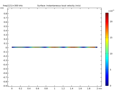
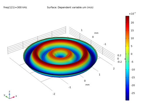
In the Settings window for Surface, click Replace Expression in the upper-right corner of the Expression section. From the menu, choose Component 1 (comp1)>Thermoviscous Acoustics, Frequency Domain>Acceleration and velocity>ta.v_inst - Instantaneous local velocity - m/s.
3
In the Velocity toolbar, click  Plot.
4
Click the  Zoom Extents button in the Graphics toolbar.
Membrane Deformation
1
In the Home toolbar, click  Add Plot Group and choose 1D Plot Group.
2
In the Settings window for 1D Plot Group, type Membrane Deformation in the Label text field.
3
Click to expand the Title section. From the Title type list, choose Label.
Line Graph 1
1
Right-click Membrane Deformation and choose Line Graph.
2
Click the  Zoom Extents button in the Graphics toolbar.
3
In the Settings window for Line Graph, locate the Selection section.
4
From the Selection list, choose Membrane.
5
Locate the y-Axis Data section. In the Expression text field, type real(U).
6
Locate the x-Axis Data section. From the Parameter list, choose Expression.
7
In the Expression text field, type r.
8
In the Membrane Deformation toolbar, click  Plot.
Pressure Under Membrane
1
In the Home toolbar, click  Add Plot Group and choose 1D Plot Group.
2
In the Settings window for 1D Plot Group, type Pressure Under Membrane in the Label text field.
3
Locate the Title section. From the Title type list, choose Label.
Line Graph 1
1
Right-click Pressure Under Membrane and choose Line Graph.
2
In the Settings window for Line Graph, locate the Selection section.
3
From the Selection list, choose Membrane.
4
Locate the y-Axis Data section. In the Expression text field, type real(p).
5
Locate the x-Axis Data section. From the Parameter list, choose Expression.
6
In the Expression text field, type r.
7
In the Pressure Under Membrane toolbar, click  Plot.
Average Membrane Velocity
1
In the Home toolbar, click  Add Plot Group and choose 1D Plot Group.
2
In the Settings window for 1D Plot Group, type Average Membrane Velocity in the Label text field.
3
Locate the Title section. From the Title type list, choose Label.
4
Locate the Plot Settings section. Select the y-axis label check box.
5
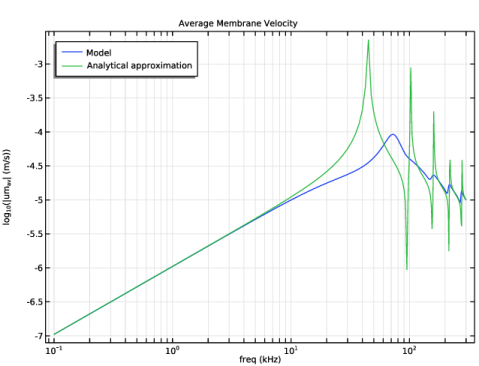
In the associated text field, type log<sub>10</sub>(|um<sub>av</sub>| (m/s)).
6
Locate the Legend section. From the Position list, choose Upper left.
Global 1
1
Right-click Average Membrane Velocity and choose Global.
2
In the Settings window for Global, locate the y-Axis Data section.
3
4
In the Average Membrane Velocity toolbar, click  Plot.
5
Click the  x-Axis Log Scale button in the Graphics toolbar.
Average Membrane Deformation
1
In the Home toolbar, click  Add Plot Group and choose 1D Plot Group.
2
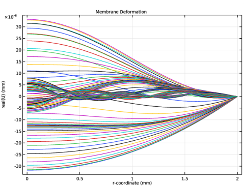
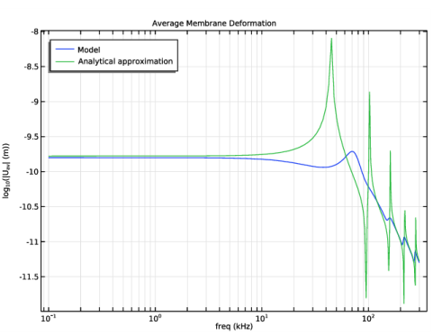
In the Settings window for 1D Plot Group, type Average Membrane Deformation in the Label text field.
3
Locate the Title section. From the Title type list, choose Label.
4
Locate the Plot Settings section. Select the y-axis label check box.
5
In the associated text field, type log<sub>10</sub>(|U<sub>av</sub>| (m)).
6
Locate the Legend section. From the Position list, choose Upper left.
Global 1
1
Right-click Average Membrane Deformation and choose Global.
2
In the Settings window for Global, locate the y-Axis Data section.
3
4
In the Average Membrane Deformation toolbar, click  Plot.
5
Click the  x-Axis Log Scale button in the Graphics toolbar.
This reproduces the average membrane velocity plot depicted in Figure 4.
Sensitivity
1
In the Home toolbar, click  Add Plot Group and choose 1D Plot Group.
2
In the Settings window for 1D Plot Group, type Sensitivity in the Label text field.
3
Locate the Title section. From the Title type list, choose Label.
Global 1
1
Right-click Sensitivity and choose Global.
2
In the Settings window for Global, locate the y-Axis Data section.
3
4
Click to expand the Legends section. Clear the Show legends check box.
5
In the Sensitivity toolbar, click  Plot.
6
Click the  x-Axis Log Scale button in the Graphics toolbar.
This should reproduce the sensitivity curve depicted in Figure 3.
Finally, create a 2D revolution dataset to plot the membrane deformation on the revolved 3D geometry.
Revolution 2D 1
In the Results toolbar, click  More Datasets and choose Revolution 2D.
3D Membrane Deformation
1
In the Results toolbar, click  3D Plot Group.
2
In the Settings window for 3D Plot Group, type 3D Membrane Deformation in the Label text field.
Surface 1
1
Right-click 3D Membrane Deformation and choose Surface.
2
In the Settings window for Surface, locate the Expression section.
3
In the Expression text field, type um.
Deformation 1
1
Right-click Surface 1 and choose Deformation.
2
In the Settings window for Deformation, locate the Expression section.
3
In the r component text field, type 0.
4
In the phi component text field, type 0.
5
In the z component text field, type um.
6
In the 3D Membrane Deformation toolbar, click  Plot.
The plot should reproduce Figure 5.