PDF

Vector Hysteresis Modeling
Introduction
This model reproduces the TEAM (Testing Electromagnetic Analysis Method) problem 32, which aims to evaluate numerical methods for the simulation of anisotropic magnetic hysteresis. A hysteretic three-limbed laminated iron core is subject to a time-varying magnetic field generated by two coils. The Jiles-Atherton material model (available in the Magnetic Fields interface) is used to simulate the response of the material, reproducing published experimental and numerical data.
Model Definition
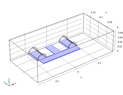
The geometry of the simulated experimental setup of TEAM problem 32 is represented in Figure 1.
Figure 1: The geometry of the device. The coils are colored in blue and the core in red.
The system is composed of a three-limbed magnetic core with two feeding coils on the two outer limbs. A low excitation frequency (10 Hz) and a finite lamination of the frame prevent skin effects in the core. The frame is composed of 5 layers with a thickness of 0.48 mm.
The applied magnetic field is mainly oriented in the xy-plane; the material is anisotropic and react differently to fields applied along the x or the y direction. In the experimental setup there are a series of pick-up coils used to accurately probe the magnetic field; these coils are not included in the model as point measurements can easily be made by means of direct numerical evaluations.
Ref. 1 details four analysis cases that differ in the applied excitations. The case represented numerically in this model is the third one, in which the two coils are excited with an AC source with a peak value of 14.5 V and in quadrature phase. The coils have a total DC resistance of 11.42 Ω which includes an externally applied resistance. The field generated by this setup is strong enough to drive the material to saturation, while the phase shift creates a rotating field at the junction between the central limb and the frame.
In the literature, experimental results have been compared favorably with vector hysteresis models (Ref. 1 and 4). This model follows Ref. 4 in using the empirical Jiles-Atherton magnetic hysteresis model to simulate the core material. The values of the parameters for the empirical model are presented in Table 1. For an anisotropic material, the parameters are all diagonal matrices; the table reports the values on the diagonal.
The Jiles-Atherton model is particularly suitable for AC feeding and requires only a limited number of parameters: a and Ms control the slope of the hysteretic B-H curve respectively at zero field and at saturation; c and k control the strength of the hysteretic effects — with the limit of no hysteresis for c = 1 or for large k. The values presented in Table 1are taken from Ref. 1 and are obtained by fitting the model to experimental data.
Results and Discussion
Figure 2 shows the magnetic flux at two different time instants, t = 275 ms (top) and t = 300 ms (bottom), at which the current in respectively the left and the right coil is at the peak value. The images show how the magnetic field rotates in the xy-plane at the junction between the central limb and the outer frame.
Figure 2: Magnetic flux density at t = 275 ms (top) and t = 300 ms (bottom).
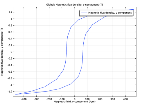
The hysteretic behavior can be displayed by plotting the magnetic flux density as a function of the magnetic field during one AC cycle (corresponding to one hysteresis loop). Figure 3 shows the hysteresis loop obtained by averaging the quantities on a cross section of the central limb.
Figure 3: Hysteresis (B-H) loop in the central limb.
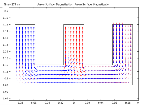
Finally, a representation of instantaneous magnetization field is shown in Figure 4. In those figures the red and blue vectors represent the instantaneous fields respectively at the time t = 300 ms and t = 275 ms, when the fields are expected to be in quadrature. The plots highlight how the fields at the junction are rotating in the xy-plane.
Figure 4: Magnetization vector field at t = 275 ms (red) and t = 300 ms (blue).
Notes About the COMSOL Implementation
The application uses the Jiles-Atherton hysteresis model available in the Magnetic Fields physics interface. The anisotropic material is constructed starting from the default isotropic Jiles-Atherton material (available in the AC/DC Module material library) and modifying the properties appropriately.
To obtain a good compromise between an accurate solution, robust convergence and efficient solving, the following settings are used:
A direct solver (PARDISO) is used instead of the default iterative solver. In order to solve a Magnetic Fields problem with a direct solver it is necessary to apply the Gauge Fixing for A-Field feature.
The discretization order for the magnetic vector potential A is set to use Linear elements. The discretization order of the Jiles-Atherton auxiliary dependent variables is then automatically set to zero.
References
1. https://www.compumag.org/wp/
2. http://www.cadema.polito.it/team32
3. A.J. Bergqvist, “A Simple Vector Generalization of the Jiles-Atherton Model of Hysteresis,” IEEE Transactions on Magnetics, vol. 32, no. 5, p. 4213, 1996.
4. J.P.A. Bastos and N. Sadowski, Magnetic Materials and 3D Finite Element Modeling, CRC Press 2014.
5. S. Yan and J.-M. Jin, “Theoretical Formulation of a Time-Domain Finite Element Method for Nonlinear Magnetic Problems in Three Dimensions,” Progress In Electromagnetics Research, vol. 153, pp. 33–55, 2015.
Application Library path: ACDC_Module/Other_Industrial_Applications/vector_hysteresis_modeling
Modeling Instructions
From the File menu, choose New.
New
In the New window, click  Model Wizard.
Model Wizard
1
In the Model Wizard window, click  3D.
2
In the Select Physics tree, select AC/DC>Electromagnetic Fields>Magnetic Fields (mf).
3
Click Add.
4
Click  Study.
5
In the Select Study tree, select Preset Studies for Selected Physics Interfaces>Coil Geometry Analysis.
6
Global Definitions
Parameters 1
1
In the Model Builder window, under Global Definitions click Parameters 1.
2
In the Settings window for Parameters, locate the Parameters section.
3
Definitions
Step 1 (step1)
1
In the Home toolbar, click  Functions and choose Global>Step.
2
In the Settings window for Step, locate the Parameters section.
3
In the Location text field, type 0.5.
4
Click to expand the Smoothing section. In the Size of transition zone text field, type 1.
Geometry 1
Work Plane 1 (wp1)
In the Geometry toolbar, click  Work Plane.
Work Plane 1 (wp1)>Plane Geometry
In the Model Builder window, click Plane Geometry.
Work Plane 1 (wp1)>Rectangle 1 (r1)
1
In the Work Plane toolbar, click  Rectangle.
2
In the Settings window for Rectangle, locate the Size and Shape section.
3
In the Width text field, type W.
4
In the Height text field, type H/2.
5
Locate the Position section. From the Base list, choose Center.
6
In the yw text field, type 3*H/4.
Work Plane 1 (wp1)>Rectangle 2 (r2)
1
In the Work Plane toolbar, click  Rectangle.
2
In the Settings window for Rectangle, locate the Size and Shape section.
3
In the Width text field, type w1.
4
In the Height text field, type h1/2.
5
Locate the Position section. From the Base list, choose Center.
6
In the xw text field, type -(w+w1)/2.
7
In the yw text field, type H-h1/4.
Work Plane 1 (wp1)>Rectangle 3 (r3)
1
In the Work Plane toolbar, click  Rectangle.
2
In the Settings window for Rectangle, locate the Size and Shape section.
3
In the Width text field, type w1.
4
In the Height text field, type h1/2.
5
Locate the Position section. From the Base list, choose Center.
6
In the xw text field, type (w+w1)/2.
7
In the yw text field, type H-h1/4.
Work Plane 1 (wp1)>Difference 1 (dif1)
1
In the Work Plane toolbar, click  Booleans and Partitions and choose Difference.
2
3
In the Settings window for Difference, locate the Difference section.
4
Find the Objects to subtract subsection. Select the  Activate Selection toggle button.
5
Select the objects r2 and r3 only.
Extrude 1 (ext1)
1
In the Model Builder window, under Component 1 (comp1)>Geometry 1 right-click Work Plane 1 (wp1) and choose Extrude.
2
In the Settings window for Extrude, locate the Distances section.
3
Cylinder 1 (cyl1)
1
In the Geometry toolbar, click  Cylinder.
2
In the Settings window for Cylinder, locate the Size and Shape section.
3
In the Radius text field, type w*0.7.
4
In the Height text field, type h1/2.
5
Locate the Position section. In the x text field, type -w-w1.
6
In the y text field, type H-h1/2.
7
Locate the Axis section. From the Axis type list, choose y-axis.
8
Click to expand the Layers section. In the table, enter the following settings:
Delete Entities 1 (del1)
1
In the Model Builder window, right-click Geometry 1 and choose Delete Entities.
2
In the Settings window for Delete Entities, locate the Entities or Objects to Delete section.
3
From the Geometric entity level list, choose Domain.
4
Click the  Zoom Extents button in the Graphics toolbar.
5
On the object cyl1, select Domains 3–5 only.
Copy 1 (copy1)
1
In the Geometry toolbar, click  Transforms and choose Copy.
2
3
In the Settings window for Copy, locate the Displacement section.
4
In the x text field, type (w+w1)*2.
Block 1 (blk1)
1
In the Geometry toolbar, click  Block.
2
In the Settings window for Block, locate the Size and Shape section.
3
In the Width text field, type 2*W.
4
In the Depth text field, type H.
5
In the Height text field, type 3*w.
6
Locate the Position section. In the x text field, type -W.
7
In the Geometry toolbar, click  Build All.
8
Click the  Zoom Extents button in the Graphics toolbar.
9
Click the  Wireframe Rendering button in the Graphics toolbar to get a better view.
Materials
Air
1
In the Model Builder window, under Component 1 (comp1) right-click Materials and choose Blank Material.
Specify the material properties for the surrounding air. A small but nonzero conductivity is required in 3D Magnetic Fields simulations to obtain consistent equations.
2
In the Settings window for Material, locate the Material Contents section.
3
4
Right-click Material 1 (mat1) and choose Rename.
5
In the Rename Material dialog box, type Air in the New label text field.
6
Coil
1
In the Model Builder window, right-click Materials and choose Blank Material.
2
3
In the Settings window for Material, locate the Material Contents section.
4
5
Right-click Material 2 (mat2) and choose Rename.
6
In the Rename Material dialog box, type Coil in the New label text field.
7
The following steps create the material for the Jiles-Atherton hysteresis model. First add the isotropic default material, then modify it to make it anisotropic.
Add Material
1
In the Home toolbar, click  Add Material to open the Add Material window.
2
Go to the Add Material window.
3
In the tree, select AC/DC>Jiles-Atherton Hysteretic Material.
4
Click  Add to Component 1 (comp1).
5
In the Home toolbar, click  Add Material to close the Add Material window.
Materials
Jiles-Atherton Hysteretic Material (mat3)
1
Start by specifying the basic material properties. Since the Jiles-Atherton model will be used for the magnetic behavior of the material it is not necessary to specify a magnetic permeability.
2
In the Settings window for Material, locate the Material Contents section.
3
Now update the parameters specific to the Jiles-Atherton model. For each parameter in the Output properties table, perform the following steps:
4
In the Model Builder window, expand the Jiles-Atherton Hysteretic Material (mat3) node, then click Jiles-Atherton model parameters (ja).
5
6
Click the Edit button below the table.
7
Choose Diagonal and enter the diagonal elements according to the following table:
8
Jiles-Atherton Isotropic Hysteretic Material
1
In the Model Builder window, under Component 1 (comp1)>Materials right-click Jiles-Atherton Hysteretic Material (mat3) and choose Rename.
2
In the Rename Material dialog box, type Jiles-Atherton Anisotropic Hysteretic Material in the New label text field.
3
Magnetic Fields (mf)
Apply a Perfect Magnetic Conductor on the antisymmetry cut to set the appropriate boundary condition (zero tangential magnetic field). The default Magnetic Insulation is the correct boundary condition for the symmetry cut boundaries (zero normal magnetic field).
Perfect Magnetic Conductor 1
1
In the Model Builder window, under Component 1 (comp1) right-click Magnetic Fields (mf) and choose Perfect Magnetic Conductor.
2
Ampère’s Law 2
1
In the Physics toolbar, click  Domains and choose Ampère’s Law.
2
It might be easier to select the correct domain by using the Selection List window. To open this window, in the Home toolbar click Windows and choose Selection List. (If you are running the cross-platform desktop, you find Windows in the main menu.)
3
In the Settings window for Ampère’s Law, locate the Constitutive Relation B-H section.
4
From the Magnetization model list, choose Hysteresis Jiles-Atherton model.
Coil 1
1
In the Physics toolbar, click  Domains and choose Coil.
2
In the Settings window for Coil, locate the Coil section.
3
From the Conductor model list, choose Homogenized multiturn.
4
From the Coil type list, choose Numeric.
5
From the Coil excitation list, choose Voltage.
6
In the Vcoil text field, type 14.5[V]*sin(2*pi*f*t)*step1(f*t).
7
Locate the Homogenized Multiturn Conductor section. In the N text field, type 90.
8
In the acoil text field, type (90*mf.coil1.length)/(6e7[S/m]*R_coil).
9
Geometry Analysis 1
1
In the Model Builder window, click Geometry Analysis 1.
2
In the Settings window for Geometry Analysis, locate the Coil Geometry section.
3
Find the Symmetry specification subsection. In the FL text field, type 2.
4
In the FA text field, type 2.
Input 1
1
In the Model Builder window, expand the Geometry Analysis 1 node, then click Input 1.
2
Geometry Analysis 1
In the Model Builder window, click Geometry Analysis 1.
Output 1
1
In the Physics toolbar, click  Attributes and choose Output.
2
Coil 2
1
In the Physics toolbar, click  Domains and choose Coil.
2
3
In the Settings window for Coil, locate the Coil section.
4
From the Conductor model list, choose Homogenized multiturn.
5
From the Coil type list, choose Numeric.
6
From the Coil excitation list, choose Voltage.
7
In the Vcoil text field, type 14.5[V]*cos(2*pi*f*t)*step1(f*t).
8
Locate the Homogenized Multiturn Conductor section. In the N text field, type 90.
9
In the acoil text field, type (90*mf.coil2.length)/(6e7[S/m]*R_coil).
Geometry Analysis 1
1
In the Model Builder window, click Geometry Analysis 1.
2
In the Settings window for Geometry Analysis, locate the Coil Geometry section.
3
Find the Symmetry specification subsection. In the FL text field, type 2.
4
In the FA text field, type 2.
Input 1
1
In the Model Builder window, expand the Geometry Analysis 1 node, then click Input 1.
2
Geometry Analysis 1
In the Model Builder window, click Geometry Analysis 1.
Output 1
1
In the Physics toolbar, click  Attributes and choose Output.
2
Apply a Gauge Fixing for A-Field feature to improve the stability of the computation and in order to use a direct solver.
Gauge Fixing for A-field 1
1
In the Physics toolbar, click  Domains and choose Gauge Fixing for A-field.
Using lower order shape functions improves the robustness of the solution process for a nonlinear problem such as the Jiles-Atherton hysteresis model. Lowering the order also reduces the size of the problem, making it easier to solve with Gauge Fixing and a direct solver.
2
In the Model Builder window, click Magnetic Fields (mf).
3
In the Settings window for Magnetic Fields, click to expand the Discretization section.
4
From the Magnetic vector potential list, choose Linear.
Mesh 1
1
In the Model Builder window, under Component 1 (comp1) click Mesh 1.
2
In the Settings window for Mesh, locate the Physics-Controlled Mesh section.
3
From the Element size list, choose Coarser.
Free Triangular 1
1
In the Mesh toolbar, click  Boundary and choose Free Triangular.
2
Size 1
1
Right-click Free Triangular 1 and choose Size.
2
In the Settings window for Size, locate the Element Size section.
3
Click the Custom button.
4
Locate the Element Size Parameters section. Select the Maximum element size check box.
5
6
Select the Maximum element growth rate check box.
7
Swept 1
1
In the Mesh toolbar, click  Swept.
2
In the Settings window for Swept, locate the Domain Selection section.
3
From the Geometric entity level list, choose Domain.
4
Distribution 1
1
Right-click Swept 1 and choose Distribution.
2
In the Settings window for Distribution, locate the Distribution section.
3
In the Number of elements text field, type 1.
Free Tetrahedral 1
1
In the Mesh toolbar, click  Free Tetrahedral.
2
In the Settings window for Free Tetrahedral, click  Build All.
Study 1
Time Dependent
1
In the Study toolbar, click  Study Steps and choose Time Dependent>Time Dependent.
2
In the Settings window for Time Dependent, locate the Study Settings section.
3
From the Time unit list, choose ms.
4
In the Output times text field, type range(0,2.5,300).
To improve the robustness and the performance of the solution, generate the default solvers and adjust some settings.
Solution 1 (sol1)
1
In the Study toolbar, click  Show Default Solver.
Set a manual scaling for the magnetic vector potential and the internal states used in the Jiles-Atherton model (magnetization and magnetic field). An appropriate value would be the maximum expected value for these quantities.
2
In the Model Builder window, expand the Solution 1 (sol1) node.
3
In the Model Builder window, expand the Study 1>Solver Configurations>Solution 1 (sol1)>Dependent Variables 2 node, then click Magnetic vector potential (comp1.A).
4
In the Settings window for Field, locate the Scaling section.
5
From the Method list, choose Manual.
6
In the Scale text field, type 5e-3.
Similarly set Scaling to Manual for the other variables with the Scaling set according to the following table.
7
8
In the Model Builder window, click Fully Coupled 1.
9
In the Settings window for Fully Coupled, locate the General section.
10
From the Linear solver list, choose Direct.
11
In the Model Builder window, click Direct.
12
In the Settings window for Direct, locate the General section.
13
From the Solver list, choose PARDISO.
14
In the Study toolbar, click  Compute.
When the computation is completed, the default plot is generated and shown. Follow these steps to replicate Figure 2.
Results
Cut Plane 1
1
In the Model Builder window, expand the Results>Datasets node, then click Cut Plane 1.
2
In the Settings window for Cut Plane, locate the Plane Data section.
3
In the z-coordinate text field, type 0.
Cut Plane 2
1
In the Model Builder window, click Cut Plane 2.
2
In the Settings window for Cut Plane, locate the Plane Data section.
3
In the x-coordinate text field, type W.
Cut Plane 3
1
In the Model Builder window, click Cut Plane 3.
2
In the Settings window for Cut Plane, locate the Plane Data section.
3
In the y-coordinate text field, type H.
Multislice 1
1
In the Model Builder window, expand the Results>Magnetic Flux Density Norm (mf) node, then click Multislice 1.
2
In the Settings window for Multislice, locate the Multiplane Data section.
3
Find the x-planes subsection. In the Coordinates text field, type W.
4
Find the y-planes subsection. In the Coordinates text field, type H.
5
Find the z-planes subsection. In the Coordinates text field, type 0.
Magnetic Flux Density Norm (mf)
1
In the Model Builder window, click Magnetic Flux Density Norm (mf).
2
In the Magnetic Flux Density Norm (mf) toolbar, click  Plot.
Next, add and set up a dedicated view that zooms in on the magnet.
3
Click the  Show More Options button in the Model Builder toolbar.
4
In the Show More Options dialog box, in the tree, select the check box for the node Results>Views.
5
View 3D 3
1
In the Model Builder window, right-click Views and choose View 3D.
2
3
In the Settings window for View 3D, locate the View section.
4
Select the Lock camera check box.
Magnetic Flux Density Norm (mf)
1
In the Model Builder window, click Magnetic Flux Density Norm (mf).
2
In the Settings window for 3D Plot Group, locate the Plot Settings section.
3
From the View list, choose View 3D 3 to apply the view you just created.
Selection 1
1
In the Model Builder window, right-click Multislice 1 and choose Selection.
2
Magnetic Flux Density Norm (mf)
Use the Time combo box to visualize the results at different times. Select 275 ms and 300 ms to reproduce Figure 2.
1
In the Model Builder window, click Magnetic Flux Density Norm (mf).
2
In the Magnetic Flux Density Norm (mf) toolbar, click  Plot.
3
In the Settings window for 3D Plot Group, locate the Data section.
4
From the Time (ms) list, choose 275.
5
In the Magnetic Flux Density Norm (mf) toolbar, click  Plot.
Create some auxiliary datasets to use in the other plots.
Cut Point 3D 1
1
In the Results toolbar, click  Cut Point 3D.
2
In the Settings window for Cut Point 3D, locate the Point Data section.
3
In the x text field, type 0.
4
In the y text field, type H-61.5[mm].
5
In the z text field, type 0.
Average 1
In the Results toolbar, click  More Datasets and choose Evaluation>Average.
Selection
1
In the Results toolbar, click  Attributes and choose Selection.
2
In the Settings window for Selection, locate the Geometric Entity Selection section.
3
From the Geometric entity level list, choose Boundary.
4
Surface 1
1
In the Results toolbar, click  More Datasets and choose Surface.
2
3
In the Settings window for Surface, locate the Parameterization section.
4
From the x- and y-axes list, choose xy-plane.
1D Plot Group 2
1
In the Results toolbar, click  1D Plot Group.
2
In the Settings window for 1D Plot Group, locate the Data section.
3
From the Dataset list, choose Cut Point 3D 1.
Point Graph 1
1
Right-click 1D Plot Group 2 and choose Point Graph.
2
In the Settings window for Point Graph, locate the y-Axis Data section.
3
In the Expression text field, type mf.By.
4
Locate the x-Axis Data section. From the Parameter list, choose Expression.
5
In the Expression text field, type mf.Bx.
6
In the 1D Plot Group 2 toolbar, click  Plot.
Rotating Field
1
In the Model Builder window, click 1D Plot Group 2.
2
In the Settings window for 1D Plot Group, locate the Data section.
3
From the Time selection list, choose Interpolated.
4
In the Times (ms) text field, type range(200,2.5,300).
5
In the 1D Plot Group 2 toolbar, click  Plot.
6
Right-click 1D Plot Group 2 and choose Rename.
7
In the Rename 1D Plot Group dialog box, type Rotating Field in the New label text field.
8
1D Plot Group 3
In the Home toolbar, click  Add Plot Group and choose 1D Plot Group.
Global 1
1
In the Model Builder window, right-click 1D Plot Group 3 and choose Global.
Plot the current flowing in the first coil.
2
In the Settings window for Global, click Replace Expression in the upper-right corner of the y-Axis Data section. From the menu, choose Component 1 (comp1)>Magnetic Fields>Coil parameters>mf.ICoil_1 - Coil current - A.
Coil Current
1
In the Model Builder window, click 1D Plot Group 3.
2
In the Settings window for 1D Plot Group, locate the Data section.
3
From the Time selection list, choose Interpolated.
4
Click  Range.
5
In the Range dialog box, type 200 in the Start text field.
6
In the Step text field, type 2.
7
In the Stop text field, type 300.
8
Click Replace.
9
In the 1D Plot Group 3 toolbar, click  Plot.
10
Right-click 1D Plot Group 3 and choose Rename.
11
In the Rename 1D Plot Group dialog box, type Coil Current in the New label text field.
12
1D Plot Group 4
In the Home toolbar, click  Add Plot Group and choose 1D Plot Group.
Global 1
1
In the Model Builder window, right-click 1D Plot Group 4 and choose Global.
In the Expression enter mf.ICoil_1-mf.VCoil_1/mf.RCoil_1.
2
In the Settings window for Global, locate the x-Axis Data section.
3
From the Parameter list, choose Frequency spectrum.
4
In the 1D Plot Group 4 toolbar, click  Plot.
Electric Current Harmonic Pollution
1
In the Model Builder window, right-click 1D Plot Group 4 and choose Rename.
2
In the Rename 1D Plot Group dialog box, type Electric Current Harmonic Pollution in the New label text field.
3
1D Plot Group 5
1
In the Home toolbar, click  Add Plot Group and choose 1D Plot Group.
2
In the Settings window for 1D Plot Group, locate the Data section.
3
From the Dataset list, choose Average 1.
4
From the Time selection list, choose Interpolated.
5
Click  Range.
6
In the Range dialog box, type 200 in the Start text field.
7
In the Step text field, type 2.
8
In the Stop text field, type 300.
9
Click Replace.
Global 1
1
Right-click 1D Plot Group 5 and choose Global.
Enter the quantities to be averaged on the boundary.
2
In the Settings window for Global, locate the y-Axis Data section.
3
4
Locate the x-Axis Data section. From the Parameter list, choose Expression.
5
In the Expression text field, type mf.Hy.
6
In the 1D Plot Group 5 toolbar, click  Plot.
Hysteresis
1
In the Model Builder window, right-click 1D Plot Group 5 and choose Rename.
2
In the Rename 1D Plot Group dialog box, type Hysteresis in the New label text field.
3
This reproduces Figure 3.
2D Plot Group 6
1
In the Home toolbar, click  Add Plot Group and choose 2D Plot Group.
2
In the Settings window for 2D Plot Group, locate the Data section.
3
From the Dataset list, choose Surface 1.
4
From the Time (ms) list, choose 275.
5
Click the  Zoom Extents button in the Graphics toolbar.
Arrow Surface 1
1
Right-click 2D Plot Group 6 and choose Arrow Surface.
2
In the Settings window for Arrow Surface, locate the Expression section.
3
In the x component text field, type mf.Mx.
4
In the y component text field, type mf.My.
5
Locate the Arrow Positioning section. Find the x grid points subsection. In the Points text field, type 41.
6
Locate the Coloring and Style section. From the Arrow type list, choose Cone.
Arrow Surface 2
1
Right-click Arrow Surface 1 and choose Duplicate.
2
In the Settings window for Arrow Surface, locate the Coloring and Style section.
3
Select the Scale factor check box.
4
5
Locate the Data section. From the Dataset list, choose Surface 1.
6
Locate the Coloring and Style section. From the Color list, choose Blue.
Arrow Surface 1
1
In the Model Builder window, click Arrow Surface 1.
2
In the Settings window for Arrow Surface, locate the Coloring and Style section.
3
Select the Scale factor check box.
4
5
In the 2D Plot Group 6 toolbar, click  Plot.
Magnetization
1
In the Model Builder window, right-click 2D Plot Group 6 and choose Rename.
2
In the Rename 2D Plot Group dialog box, type Magnetization in the New label text field.
3
This reproduces Figure 4. Plot the magnetic field as a vector field to visualize the rotation of the field at the junction.
Magnetic Field
1
Right-click Magnetization and choose Duplicate.
2
Right-click Magnetization 1 and choose Rename.
3
In the Rename 2D Plot Group dialog box, type Magnetic Field in the New label text field.
4
Arrow Surface 1
1
In the Model Builder window, expand the Magnetic Field node, then click Arrow Surface 1.
2
In the Settings window for Arrow Surface, locate the Expression section.
3
In the x component text field, type mf.Hx.
4
In the y component text field, type mf.Hy.
5
Locate the Coloring and Style section. In the Scale factor text field, type 2e-5.
Arrow Surface 2
1
In the Model Builder window, click Arrow Surface 2.
2
In the Settings window for Arrow Surface, locate the Expression section.
3
In the x component text field, type mf.Hx.
4
In the y component text field, type mf.Hy.
5
Locate the Coloring and Style section. In the Scale factor text field, type 2e-5.
6
In the Magnetic Field toolbar, click  Plot.