|
|
|

|
1
|
|
2
|
Browse to the model’s Application Libraries folder and double-click the file submarine_cable_04_inductive_effects.mph.
|
|
3
|
|
4
|
Browse to a suitable folder and type the filename submarine_cable_06_thermal_effects.mph.
|
|
1
|
In the Model Builder window, expand the Component 1 (comp1)>Magnetic Fields (mf) node, then click Phase 1.
|
|
2
|
Click to collapse the Material Type section, the Coordinate System Selection section, and the Constitutive Relation sections.
|
|
3
|
|
4
|
|
1
|
|
2
|
|
3
|
|
4
|
Browse to the model’s Application Libraries folder and double-click the file submarine_cable_d_therm_parameters.txt.
|
|
1
|
|
2
|
|
3
|
|
4
|
|
5
|
|
1
|
|
2
|
|
3
|
|
1
|
|
2
|
|
3
|
|
4
|
|
5
|
|
1
|
|
2
|
|
3
|
|
1
|
|
2
|
|
3
|
Find the Studies subsection. In the Select Study tree, select Preset Studies for Selected Multiphysics>Frequency-Stationary.
|
|
4
|
|
5
|
|
1
|
|
2
|
|
1
|
In the Model Builder window, expand the Component 1 (comp1)>Materials node, then click Copper (mat11).
|
|
2
|
|
1
|
In the Model Builder window, under Component 1 (comp1)>Materials right-click Air (mat1) and choose Duplicate.
|
|
2
|
|
3
|
Locate the Geometric Entity Selection section. From the Geometric entity level list, choose Boundary.
|
|
4
|
|
5
|
|
1
|
|
2
|
|
3
|
|
4
|
Locate the Shell Properties section. From the Shell type list, choose Nonlayered shell. In the Lth text field, type 20[um].
|
|
1
|
|
2
|
|
4
|
|
5
|
|
1
|
|
2
|
|
3
|
|
4
|
|
1
|
|
2
|
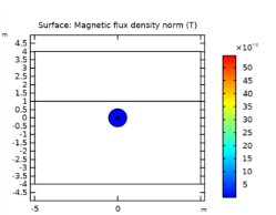
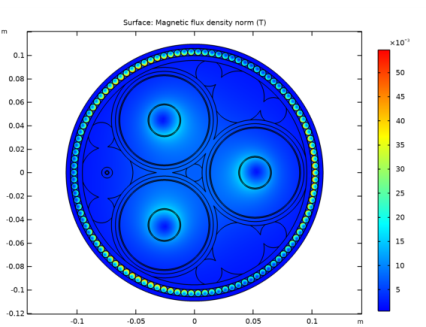
In the Settings window for 2D Plot Group, type Magnetic Flux Density Norm (mf) in the Label text field.
|
|
1
|
|
2
|
|
3
|
|
4
|
|
1
|
|
2
|
|
3
|
|
4
|
|
5
|
|
1
|
|
2
|
|
3
|
|
4
|
|
5
|
|
1
|
|
2
|
|
3
|
|
4
|
|
1
|
|
2
|
|
3
|
|
4
|
|
5
|
|
6
|
|
7
|
|
8
|
|
1
|
|
2
|
|
3
|
|
4
|
|
5
|
|
6
|
|
1
|
|
2
|
|
3
|
|
4
|
|
5
|
Locate the Expressions section. In the table, enter the following settings. That is; replace “W/m” (the default) with “W/km”, and “2.5D+milliken” with “one-way ih”:
|
|
6
|
Click
|
|
1
|
Go to the Table window.
|
|
1
|
|
2
|
|
3
|
|
4
|
|
5
|
Locate the Expressions section. In the table, enter the following settings:
|
|
6
|
Click
|
|
1
|
Go to the Table window.
|
|
1
|
|
2
|
|
3
|
|
4
|
|
5
|
Locate the Expressions section. In the table, enter the following settings:
|
|
6
|
Click
|
|
1
|
Go to the Table window.
|
|
1
|
|
2
|
|
3
|
|
1
|
In the Model Builder window, under Component 1 (comp1)>Materials, add the following material properties:
|
|
1
|
|
2
|
|
3
|
In the table, update the description. Type Phase losses (linres phases), that is; replace “one-way ih” with “linres phases”.
|
|
4
|
|
1
|
Go to the Table window.
|
|
1
|
|
2
|
|
3
|
|
1
|
|
2
|
|
3
|
|
4
|
Click to collapse the Material Type section, the Coordinate System Selection section, the Constitutive Relation B-H section, and the Constitutive Relation D-E section.
|
|
5
|
Locate the Constitutive Relation Jc-E section. From the Conduction model list, choose Linearized resistivity.
|
|
1
|
|
2
|
|
3
|
|
1
|
|
2
|
|
3
|
In the table, update the description. Type Phase losses (coupled ih), that is; replace “linres phases” with “coupled ih”.
|
|
4
|
|
1
|
Go to the Table window.
|
|
1
|
|
2
|
|
3
|
|
4
|
Locate the Expressions section. In the table, enter the following settings. That is; replace “Ω/m” (the default) with “mohm/km”, replace “2.5D+milliken” with “coupled ih”, and rewrite the row for Rcon altogether:
|
|
5
|
Click
|
|
1
|
|
2
|
|
3
|
|
4
|
Locate the Expressions section. In the table, enter the following settings. That is; replace “H/m” (the default) with “mH/km”, and “2.5D+milliken” with “coupled ih”:
|
|
5
|
Click
|
|
6
|
Go to the Table window.
|
|
1
|
|
2
|
|
3
|
|
1
|
|
2
|
|
3
|
|
4
|
Locate the Expressions section. In the table, enter the following settings:
|
|
5
|
Click
|
|
6
|
|
7
|
Locate the Expressions section. In the table, update the description. Type Temperature (screens), that is; replace “phases” with “screens”.
|
|
8
|
Click
|
|
9
|
|
10
|
In the table, update the description. Type Temperature (armor), that is; replace “screens” with “armor”.
|
|
11
|
Click
|
|
12
|
Go to the Table window.
|
|
1
|
|
2
|
|
3
|
|
1
|
|
2
|
|
3
|
|
4
|
|
5
|
|
6
|
|
7
|
|
8
|
|
9
|
|
1
|
|
2
|
|
3
|
|
4
|
|
5
|
|
1
|
In the Model Builder window, under Component 1 (comp1)>Global ODEs and DAEs (ge) click Global Equations 1.
|
|
2
|
|
4
|
|
5
|
In the Dependent variable quantity table, enter the following settings:
|
|
6
|
|
7
|
In the Source term quantity table, enter the following settings:
|
|
1
|
|
2
|
In the Show More Options dialog box, in the tree, select the check box for the node Physics>Advanced Physics Options.
|
|
3
|
Click OK.
|
|
1
|
In the Model Builder window, under Component 1 (comp1)>Global ODEs and DAEs (ge) click Global Equations 1.
|
|
2
|
|
3
|
|
1
|
|
2
|
|
3
|
|
4
|
|
5
|
|
1
|
|
2
|
|
3
|
|
1
|
|
2
|
|
3
|
In the table, update the description. Type Phase losses (preset Rac), that is; replace “coupled ih” with “preset Rac”.
|
|
4
|
|
1
|
Go to the Table window.
|
|
1
|
|
2
|
|
3
|
In the table, enter the following settings. That is; replace “coupled ih” with “preset Rac”, and remove the second row alogether:
|
|
4
|
Click
|
|
1
|
|
2
|
|
3
|
In the table, update the description. Type Phase inductance (preset Rac), that is; replace “coupled ih” with “preset Rac”.
|
|
4
|
|
5
|
Go to the Table window.
|