PDF

Inductance of a Power Inductor
Introduction
Power inductors are a central part of many low-frequency power applications. They are, for example, used in switched power supplies and DC-DC converters. The inductor is used in conjunction with a high-power semiconductor switch that operates at a certain frequency, stepping up or down the voltage on the output. The relatively low voltage and high power consumption put high demands on the design of the power supply and especially on the inductor, which must be designed with respect to switching frequency, current rating, and hot environments.
A power inductor usually has a magnetic core to increase its inductance value, reducing the demands for a high frequency while keeping the sizes small. The magnetic core also reduces the electromagnetic interference with other devices. There are only crude analytical formulas or empirical formulas available for calculating impedances, so computer simulations or measurements are necessary in the design of these inductors. This application uses a design drawn in an external CAD software, imports the geometry to COMSOL Multiphysics, and finally calculates the inductance from the specified material parameters and frequency.
Model Definition
The application uses the Magnetic and Electric Fields interface, taking electric and magnetically induced currents into account. This formulation, often referred to as an AV-formulation, solves both for the magnetic vector potential A and the electric potential V. The model is solved first with a free gauge, using an iterative, residual minimizing method and, in a second step with the Coulomb gauge
applied to the magnetic vector potential. See the Theory of Magnetic Fields and Gauge Fixing for A-field sections in the AC/DC Module User’s Guide for more details.
For very high frequencies capacitive effects yield a frequency-dependent coil reactance as shown in the related example described in the manual Introduction to AC/DC Module. There it is also shown how to handle a very small skin depth by, instead of volumetric meshing, using an asymptotic high frequency impedance boundary condition.
In this model the frequency is much lower and the coil is almost purely inductive with an inductance that is close to that computed in the static limit. Still the resistance is frequency dependent due to skin effect. Volumetric meshing is applied but with the twist of using a boundary layer mesh to resolve the skin depth.
The following table lists the material properties used in this application:
σ
5.997·107 S/m
εr
μr
103-10i
The losses in the copper coil are purely resistive, while the core loss is described using a complex relative permeability. The latter information is commonly provided by magnetic material (for example ferrites) manufacturers. In COMSOL Multiphysics the value can easily be made frequency or temperature dependent if needed by means of using interpolation tables, and so on.
The outer boundaries are mainly the default magnetic insulation and electric insulation,
The copper winding is grounded in one end. The other end uses a Terminal boundary condition to apply an electric potential of 1 V. The Terminal generates an admittance variable for the inductor that can be accessed in postprocessing. You can calculate the inductance from the formula
where ω is the angular frequency, and Y11 is the coil/Terminal admittance. The effective conductance that is due to resistive losses in the coil and magnetic losses in the core is evaluated as the real part of Y11.
Results and Discussion
The model is solved for a frequency of 1 kHz. It yields an inductance of 115 μH similar to the static value computed in the manual Introduction to AC/DC Module. The conductance evaluates to 0.015 S and is shown to be balanced by losses in model. Figure 1 shows the distribution of the real part of the electric potential distribution for the case with the Coulomb gauge applied. Note that the electric potential is not gauge invariant so it will look different with the free gauge. Only the electric and magnetic fields are independent of the gauge.
Figure 2 shows the magnetic flux density, both its norm as a slice plot and its local direction and strength at zero phase as an arrow plot.
Figure 1: Real part of the electric potential distribution.
Figure 2: The final plot of the power inductor, showing the potential on the coil, the magnitude of the flux density inside the ferrite core, and the direction of the same as arrows.
Application Library path: ACDC_Module/Inductive_Devices_and_Coils/power_inductor
Modeling Instructions
From the File menu, choose New.
New
In the New window, click  Model Wizard.
Model Wizard
1
In the Model Wizard window, click  3D.
2
In the Select Physics tree, select AC/DC>Electromagnetic Fields>Vector Formulations>Magnetic and Electric Fields (mef).
3
Click Add.
4
Click  Study.
5
In the Select Study tree, select General Studies>Frequency Domain.
6
Geometry 1
The geometry of the inductor is available as a CAD file. Import it and create a surrounding air box.
Import 1 (imp1)
1
In the Home toolbar, click  Import.
2
In the Settings window for Import, locate the Import section.
3
Click Browse.
4
5
Click Import.
Block 1 (blk1)
1
In the Geometry toolbar, click  Block.
2
In the Settings window for Block, locate the Size and Shape section.
3
In the Width text field, type 0.2.
4
In the Depth text field, type 0.15.
5
In the Height text field, type 0.12.
6
Locate the Position section. In the x text field, type -0.1.
7
In the y text field, type -0.08.
8
In the z text field, type -0.04.
9
Click  Build All Objects.
10
Click the  Wireframe Rendering button in the Graphics toolbar.
Materials
This application uses two materials that are already available in the Material Library and one defined from a Blank material.
Add Material
1
In the Home toolbar, click  Add Material to open the Add Material window.
2
Go to the Add Material window.
3
In the tree, select Built-in>Copper.
4
Click Add to Component in the window toolbar.
5
6
Click Add to Component in the window toolbar.
7
In the Home toolbar, click  Add Material to close the Add Material window.
Materials
Copper (mat1)
1
In the Model Builder window, under Component 1 (comp1)>Materials click Copper (mat1).
2
In the Settings window for Material, locate the Geometric Entity Selection section.
3
Click  Clear Selection.
4
Air (mat2)
1
In the Model Builder window, click Air (mat2).
2
Magnetic and Electric Fields (mef)
Proceed now with the setup of the physics interface and set up the Terminal and Ground conditions driving the current through the model.
Magnetic Insulation 1
In the Model Builder window, expand the Component 1 (comp1)>Magnetic and Electric Fields (mef)>Magnetic Insulation 1 node, then click Magnetic Insulation 1.
Ground 1
1
In the Physics toolbar, click  Attributes and choose Ground.
2
Magnetic Insulation 1
In the Model Builder window, click Magnetic Insulation 1.
Terminal 1
1
In the Physics toolbar, click  Attributes and choose Terminal.
2
3
In the Settings window for Terminal, locate the Terminal section.
4
From the Terminal type list, choose Voltage.
In order to model a finite loss core, it is added a constitutive relationship where the complex relative permeability is specified with the corresponding material providing these data.
Ampère’s Law and Current Conservation 2
1
In the Physics toolbar, click  Domains and choose Ampère’s Law and Current Conservation.
2
3
In the Settings window for Ampère’s Law and Current Conservation, locate the Constitutive Relation B-H section.
4
From the Magnetization model list, choose Magnetic losses.
Materials
Core Material
1
In the Model Builder window, under Component 1 (comp1) right-click Materials and choose Blank Material.
2
Right-click Material 3 (mat3) and choose Rename.
3
In the Rename Material dialog box, type Core Material in the New label text field.
4
5
6
In the Settings window for Material, locate the Material Contents section.
7
Mesh 1
1
In the Model Builder window, under Component 1 (comp1) click Mesh 1.
2
In the Settings window for Mesh, locate the Physics-Controlled Mesh section.
3
From the Element size list, choose Extra coarse.
Size
Right-click Component 1 (comp1)>Mesh 1 and choose Edit Physics-Induced Sequence.
Free Tetrahedral 1
As in the following linear elements are going to be chosen, a finer mesh in the core is added even though this is unnecessary for the first solution where default quadratic elements are used.
Size 1
1
In the Model Builder window, right-click Free Tetrahedral 1 and choose Size.
2
In the Settings window for Size, locate the Geometric Entity Selection section.
3
From the Geometric entity level list, choose Domain.
4
5
Locate the Element Size section. Click the Custom button.
6
Locate the Element Size Parameters section. Select the Maximum element size check box.
7
A boundary layer mesh is added in order to resolve skin depth.
Boundary Layers 1
1
In the Mesh toolbar, click  Boundary Layers.
2
In the Settings window for Boundary Layers, locate the Geometric Entity Selection section.
3
From the Geometric entity level list, choose Domain.
4
Boundary Layer Properties
1
In the Model Builder window, click Boundary Layer Properties.
2
3
In the Settings window for Boundary Layer Properties, locate the Boundary Layer Properties section.
4
In the Number of boundary layers text field, type 2.
5
From the Thickness of first layer list, choose Manual.
6
In the Thickness text field, type 1[mm].
7
Click  Build All.
Study 1
Step 1: Frequency Domain
1
In the Model Builder window, under Study 1 click Step 1: Frequency Domain.
2
In the Settings window for Frequency Domain, locate the Study Settings section.
3
In the Frequencies text field, type 1[kHz].
The model is now ready for solving. In order to compute the admittance with sufficient accuracy in this case with fairly low frequency, the error estimate must be increased so that the iterative solver will refine the solution more than the standard value.
Solution 1 (sol1)
1
In the Study toolbar, click  Show Default Solver.
2
In the Model Builder window, expand the Solution 1 (sol1) node.
3
In the Model Builder window, expand the Study 1>Solver Configurations>Solution 1 (sol1)>Stationary Solver 1 node, then click Iterative 1.
4
In the Settings window for Iterative, click to expand the Error section.
5
In the Factor in error estimate text field, type 1e7.
6
In the Model Builder window, click Study 1.
7
In the Settings window for Study, locate the Study Settings section.
8
Clear the Generate default plots check box.
9
In the Study toolbar, click  Compute.
Results
3D Plot Group 1
In the Home toolbar, click  Add Plot Group and choose 3D Plot Group.
Slice 1
1
Right-click 3D Plot Group 1 and choose Slice.
2
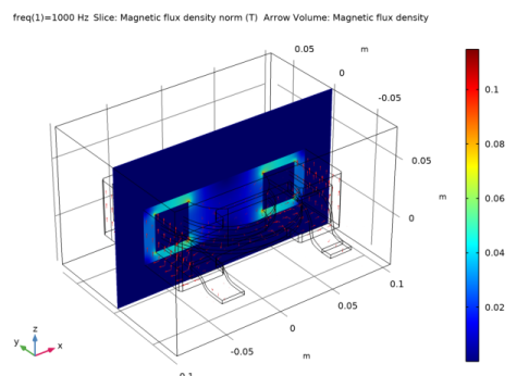
In the Settings window for Slice, click Replace Expression in the upper-right corner of the Expression section. From the menu, choose Component 1 (comp1)>Magnetic and Electric Fields>Magnetic>mef.normB - Magnetic flux density norm - T.
3
Locate the Plane Data section. From the Plane list, choose zx-planes.
4
In the Planes text field, type 1.
5
In the 3D Plot Group 1 toolbar, click  Plot.
Arrow Volume 1
1
In the Model Builder window, right-click 3D Plot Group 1 and choose Arrow Volume.
2
In the Settings window for Arrow Volume, click Replace Expression in the upper-right corner of the Expression section. From the menu, choose Component 1 (comp1)>Magnetic and Electric Fields>Magnetic>mef.Bx,...,mef.Bz - Magnetic flux density.
3
Locate the Arrow Positioning section. Find the x grid points subsection. In the Points text field, type 20.
4
Find the y grid points subsection. In the Points text field, type 20.
5
Find the z grid points subsection. In the Points text field, type 10.
6
In the 3D Plot Group 1 toolbar, click  Plot.
The plot should now look like Figure 2 .
Next instructions show how to extract the conductance and inductance.
Global Evaluation 1
1
In the Results toolbar, click  Global Evaluation.
Compute the conductance as real part of admittance, and inductance as the inverse of admittance imaginary part divided by the angular frequency. Specify the output unit as uH (microhenry, μH).
2
In the Settings window for Global Evaluation, locate the Expressions section.
3
4
Click  Evaluate.
Table
1
Go to the Table window.
Real part of admittance evaluates to about 0.015[S] while inductance 115[uH] similarly to the static limit.
Results
Finite value of real part of inductance is due to losses in the material. In the present case, most of the losses are in the lossy core, but some are also in the conducting coil. In the next it is shown how effective conductance of the coil as evaluated by the terminal is consistent with the balance of losses in the whole system.
Volume Integration 1
1
In the Results toolbar, click  More Derived Values and choose Integration>Volume Integration.
2
3
In the Settings window for Volume Integration, locate the Expressions section.
4
5
Click  Evaluate (Table 1 - Global Evaluation 1).
Magnetic and Electric Fields (mef)
In the following it is shown that an alternative to increasing solver tolerances is add gauge fixing. Gauge fixing is compatible with direct solver which essentially does not require any tuning. As direct solver implies a considerably higher computational burden, in the next, linear element are chosen. The logical step are then, adding the Gauge Fixing node, set solver to Direct, and solve. In the following this is done, but first a modified label is added to the former solver and the new one.
Gauge Fixing for A-field 1
In the Physics toolbar, click  Domains and choose Gauge Fixing for A-field.
Study 1
Model without gauge fixing - default iterative solver tweaked
1
In the Model Builder window, under Study 1>Solver Configurations click Solution 1 (sol1).
2
In the Settings window for Solution, type Model without gauge fixing - default iterative solver tweaked in the Label text field.
Model with gauge fixing - direct solver
1
In the Study toolbar, click  Show Default Solver.
2
In the Model Builder window, expand the Solution 2 (sol2) node.
3
In the Model Builder window, expand the Study 1>Solver Configurations>Solution 2 (sol2)>Stationary Solver 1 node.
4
Right-click Direct and choose Enable.
5
In the Model Builder window, click Solution 2 (sol2).
6
In the Settings window for Solution, type Model with gauge fixing - direct solver in the Label text field.
Magnetic and Electric Fields (mef)
1
In the Model Builder window, under Component 1 (comp1) click Magnetic and Electric Fields (mef).
2
In the Settings window for Magnetic and Electric Fields, click to expand the Discretization section.
3
From the Magnetic vector potential list, choose Linear.
4
From the Electric potential list, choose Linear.
Study 1
Model with gauge fixing - direct solver (sol2)
In the Model Builder window, under Study 1>Solver Configurations right-click Model with gauge fixing - direct solver (sol2) and choose Compute.
Results
Next compute the new estimate of conductance and inductance, and update the former plot.
Global Evaluation 1
1
In the Model Builder window, under Results>Derived Values click Global Evaluation 1.
2
In the Settings window for Global Evaluation, locate the Data section.
3
From the Dataset list, choose Study 1/Model with gauge fixing - direct solver (sol2).
4
Click  Evaluate (Table 1 - Global Evaluation 1).
3D Plot Group 1
1
In the Model Builder window, click 3D Plot Group 1.
2
In the Settings window for 3D Plot Group, locate the Data section.
3
From the Dataset list, choose Study 1/Model with gauge fixing - direct solver (sol2).
4
In the 3D Plot Group 1 toolbar, click  Plot.
Finally visualize the potential distribution in a new plot group.
3D Plot Group 2
1
In the Home toolbar, click  Add Plot Group and choose 3D Plot Group.
2
In the Settings window for 3D Plot Group, locate the Data section.
3
From the Dataset list, choose Study 1/Model with gauge fixing - direct solver (sol2).
Surface 1
Right-click 3D Plot Group 2 and choose Surface.
Take a look inside by hiding a few of the exterior boundaries.
Selection 1
1
In the Model Builder window, right-click Surface 1 and choose Selection.
2
Select Boundaries 3 and 5–79 only. The quickest way to do this is to select All boundaries from the Selection list, then remove Boundaries 1, 2, and 4.
3D Plot Group 2
Click 3D Plot Group 2 to visualize the plot reproducing Figure 1 .
1
In the Model Builder window, click 3D Plot Group 2.
2
In the 3D Plot Group 2 toolbar, click  Plot.
3